Data Visualization and Sentiment Analysis On Trending Youtube Statistics
Data Introduction & Processing
This dataset is from Kaggle, and it is about the trending Youtube statistics in the U.S. with more than 40000 rows and 16 columns.
After loading the tidyverse library, we can take a peek on what the dataset looks like.
library(tidyverse)
yb <- read_csv("data\\USvideos.csv")
head(yb)
## # A tibble: 6 x 16
## video_id trending_date title channel_title category_id publish_time
## <chr> <chr> <chr> <chr> <dbl> <dttm>
## 1 2kyS6SvS~ 17.14.11 WE WANT~ CaseyNeistat 22 2017-11-13 17:13:01
## 2 1ZAPwfrt~ 17.14.11 The Tru~ LastWeekToni~ 24 2017-11-13 07:30:00
## 3 5qpjK5Dg~ 17.14.11 Racist ~ Rudy Mancuso 23 2017-11-12 19:05:24
## 4 puqaWrEC~ 17.14.11 Nickelb~ Good Mythica~ 24 2017-11-13 11:00:04
## 5 d380meD0~ 17.14.11 I Dare ~ nigahiga 24 2017-11-12 18:01:41
## 6 gHZ1Qz0K~ 17.14.11 2 Weeks~ iJustine 28 2017-11-13 19:07:23
## # ... with 10 more variables: tags <chr>, views <dbl>, likes <dbl>,
## # dislikes <dbl>, comment_count <dbl>, thumbnail_link <chr>,
## # comments_disabled <lgl>, ratings_disabled <lgl>,
## # video_error_or_removed <lgl>, description <chr>While exploring the dataset, one thing we have noticed is that category_id column should be a factor column rather than a double one, as we need to group by this column to see the average statistics category-wise.
yb$category_id <- factor(yb$category_id)Data Visualization
Now it would be interesting to visualize the average likes and dislikes etc. across different categories.
yb %>% group_by(category_id) %>%
  summarize(`Average Views` = mean(views), `Average Likes` = mean(likes), `Average Dislikes` = mean(dislikes), `Average Number Of Comments` = mean(comment_count)) %>%
  pivot_longer(!category_id, names_to = "popularity", values_to = "Counts") %>%
  ggplot(aes(category_id, Counts, fill = category_id)) +
  geom_bar(stat = "identity") +
  facet_wrap(~popularity, scales = "free") +
  theme_bw() +
  theme(
    strip.text = element_text(size = 16),
    legend.position = "none",
    axis.ticks = element_blank(),
    axis.title = element_text(size = 15),
    axis.text = element_text(size = 13),
    plot.title = element_text(size = 18)
  ) +
  ggtitle("Category-wise Trending Youtube Statistics")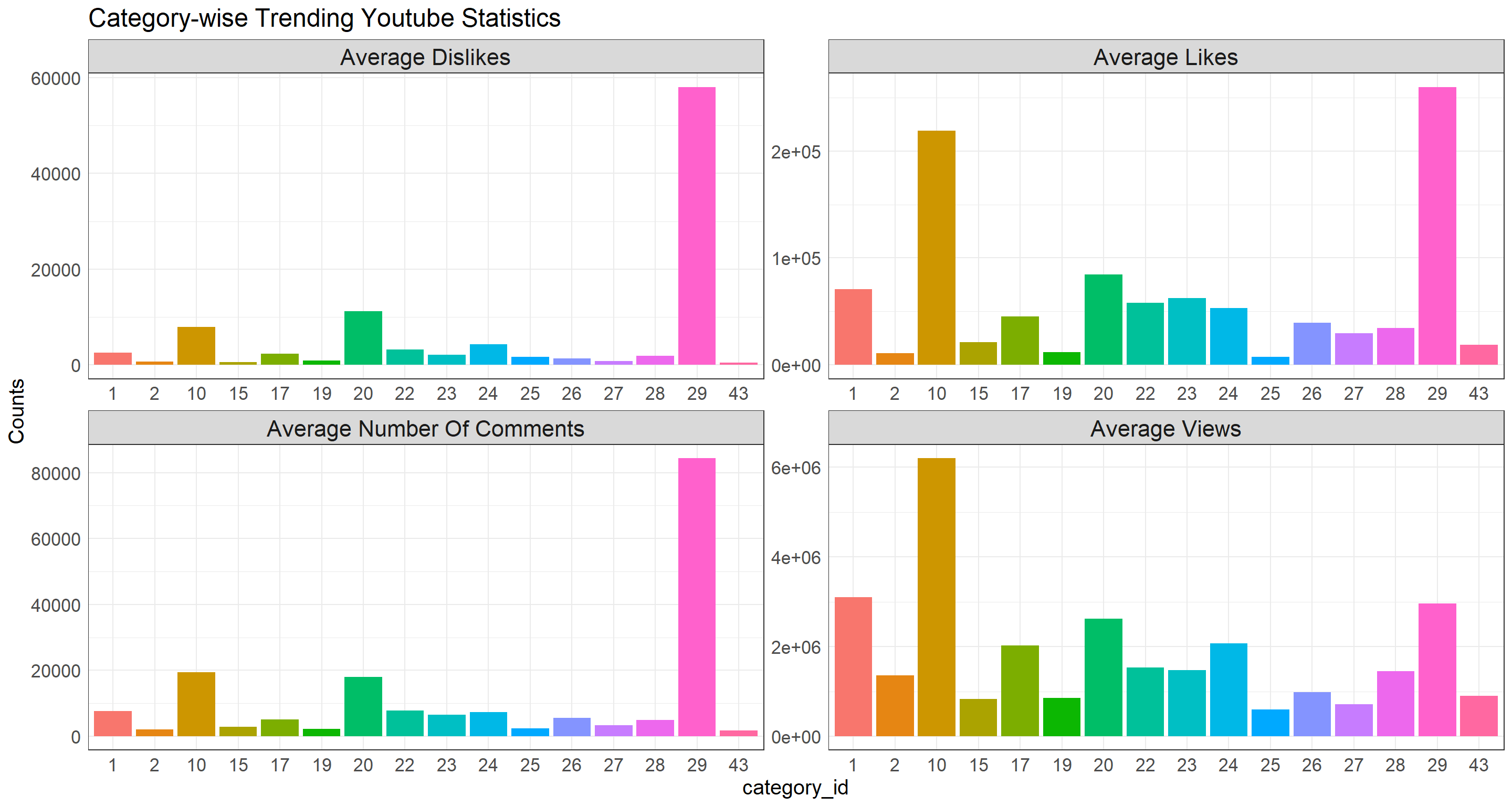
Although the dataset does not say specifically what each category_id corresponds to which video topic, but based on the bar plots above, category_id = 29 attracted much more attention (likes, dislikes, comments) on average yet the average views do not stand out at all. It seems like youtube viewers do not watch these videos but give their opinions excessively!
Let’s dive into this specific category.
yb %>% filter(category_id == 29) %>%
  ggplot(aes(row.names(yb %>% filter(category_id == 29)), comment_count)) +
    geom_bar(stat = "identity") +
  labs(x = "video index", y = "comment counts")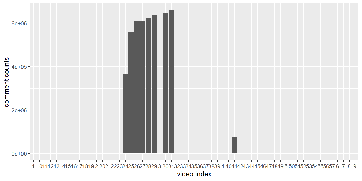
As we can see, there are few outliers in category_id = 29 that have attracted a slew of attentions and comments, yet the rest of them are barely watched by viewers.
Sentiment Analysis
There are two columns (tags and description) in the dataset where we can apply sentiment analysis. Since videos are categorized by their category ID, it is worth to see what sentiment each video category possesses by using three sentiment dictionaries (AFINN, Bing, NRC) built in the sentiment library tidytext.
library(tidytext)Here we write a function that can generate bar charts for sentiment score grouped by category_id faceted by each dictionary.
sentiment_barplots <- function(text_column, plot_title){
  text_column = enquo(text_column)
  bind_rows(
  yb %>% select(category_id, !!text_column)%>%
    unnest_tokens(word, !!text_column) %>%
    anti_join(stop_words) %>%
    inner_join(get_sentiments("afinn"))%>%
    group_by(category_id) %>%
    summarize(score = sum(value)) %>%
    mutate(method = "AFINN"),
   bind_rows(
    yb%>% select(category_id, !!text_column) %>%
      unnest_tokens(word, !!text_column) %>%
      anti_join(stop_words) %>%
      inner_join(get_sentiments("bing")) %>%
      group_by(category_id) %>%
      count(sentiment) %>%
      pivot_wider(names_from = sentiment,
                  values_from = n,
                  values_fill = 0) %>%
      mutate(score = positive - negative) %>%
      mutate(method = "Bing et al."),
    yb%>% select(category_id, !!text_column) %>%
      unnest_tokens(word, !!text_column) %>%
      anti_join(stop_words) %>%
      inner_join(get_sentiments("nrc")) %>%
      group_by(category_id) %>%
      count(sentiment) %>%
      pivot_wider(names_from = sentiment,
                  values_from = n,
                  values_fill = 0) %>%
      mutate(score = positive - negative) %>%
      select(category_id, negative, positive, score) %>%
      mutate(method = "NRC")
  ) %>%
    select(category_id, score, method)
) %>%
  ggplot(aes(category_id, score)) +
  geom_bar(aes(fill= method), stat = "identity") +
  facet_wrap(~method, ncol = 1, scales = "free") +
  theme_bw() +
  labs(x = "Video Category", y = "Sentiment Score", title = plot_title) +
  theme(legend.position = "none",
        strip.text = element_text(size = 16),
        axis.title = element_text(size = 16),
        axis.text = element_text(size = 15),
        axis.ticks = element_blank(),
        plot.title = element_text(size = 18))
}
sentiment_barplots(tags, "Tags Sentiment Score")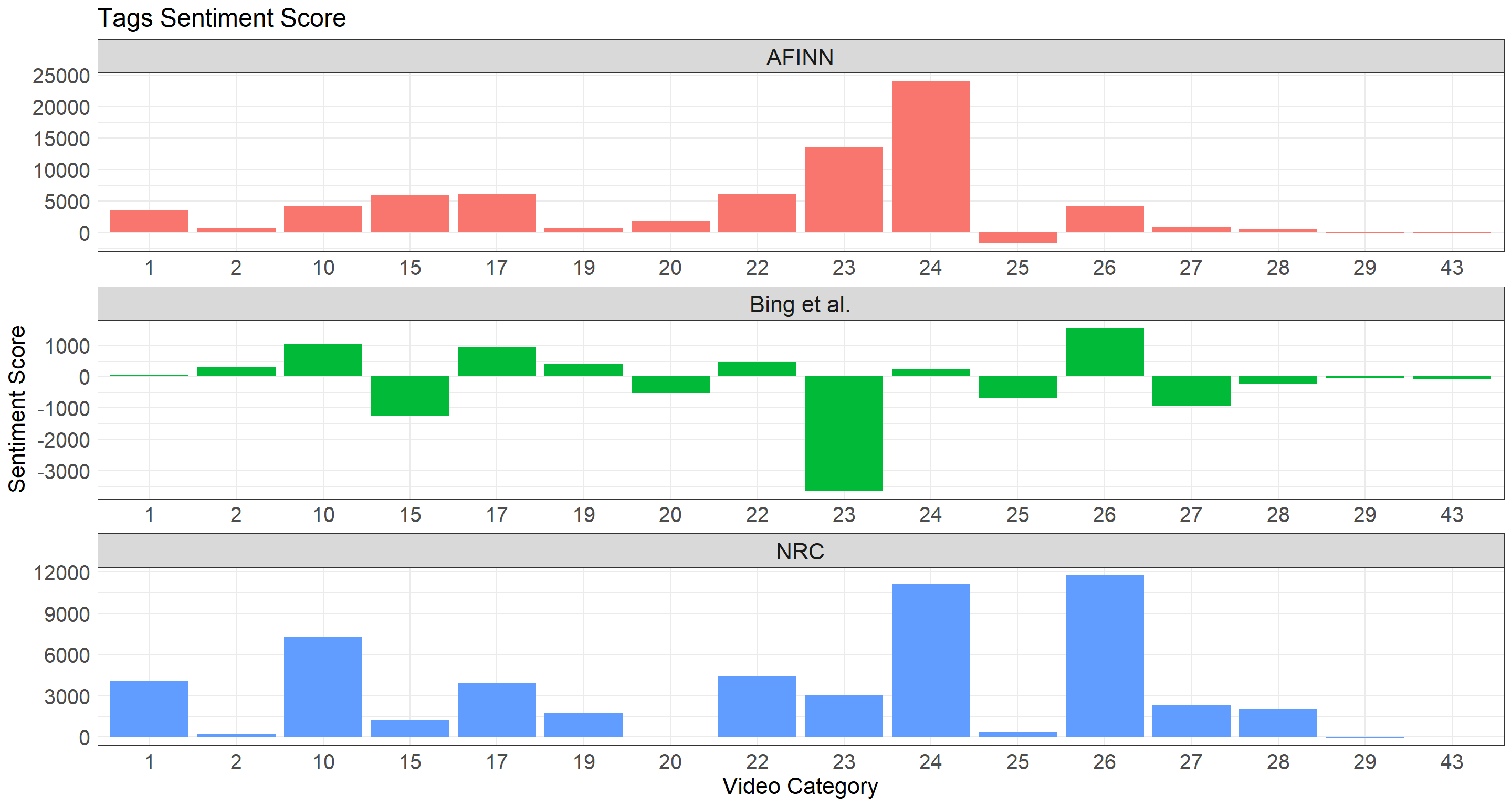
sentiment_barplots(description, "Description Sentiment Score")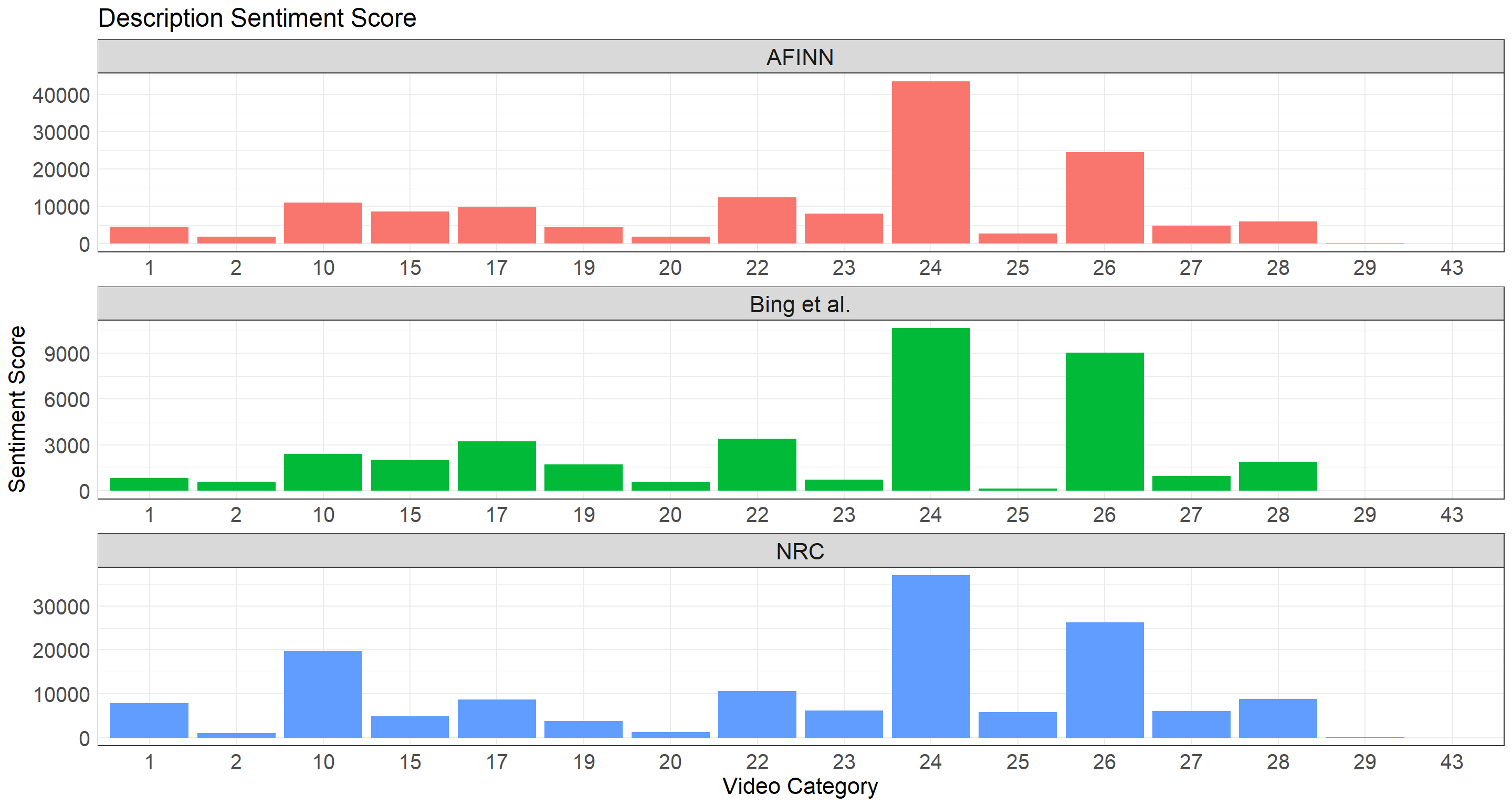
Sentiment Analysis Conclusion
When looking at Tag Sentiment Score barplot, an interesting thing to note is that bing dictionary outputs some negative sentiment scores for some categories, yet the other two only have non-negative scores. There is some inconsistency in this regard. In other words, using tags as a way to analyze video sentiment might not be a good idea due to the fact that tags are usually short and do not cover the whole picture of videos try to convey to viewers. Video description, however, offers a good consistency among all three dictionaries in a way that the sentiment scores are highly analogous.