Amazon Bestsellers Data Exploration and Category Classification
Introduction
This dataset is about Amazon Bestsellers between 2009 and 2019 from Kaggle with 50 books every year along with information related to each book (ratings, author(s) and pricing, etc.). It would be interesting to dive into this dataset to visualize it and use some machine learning algorithms to predict the bestsellers’ rating based on some selected features.
Data Exploration and Visualization
Load the libraries and dataset.
library(tidyverse)
library(caret)
library(randomForest)
books <- read_csv("bestsellers with categories.csv")
dim(books)## [1] 550 7head(books)## # A tibble: 6 x 7
## Name Author `User Rating` Reviews Price Year Genre
## <chr> <chr> <dbl> <dbl> <dbl> <dbl> <chr>
## 1 10-Day Green Smoothie C~ JJ Smith 4.7 17350 8 2016 Non F~
## 2 11/22/63: A Novel Stephen King 4.6 2052 22 2011 Ficti~
## 3 12 Rules for Life: An A~ Jordan B. P~ 4.7 18979 15 2018 Non F~
## 4 1984 (Signet Classics) George Orwe~ 4.7 21424 6 2017 Ficti~
## 5 5,000 Awesome Facts (Ab~ National Ge~ 4.8 7665 12 2019 Non F~
## 6 A Dance with Dragons (A~ George R. R~ 4.4 12643 11 2011 Ficti~First thing that comes to my mind is Genre column, as I’d like to transform it into factor in a way that 0 represents non-fiction and 1 otherwise.
books <- books %>%
  mutate(Genre_fct = case_when(Genre == "Non Fiction" ~ "0",
            Genre == "Fiction" ~ "1"))

books$Genre_fct <- as.factor(books$Genre_fct)
books$Year <- as.integer(books$Year)
This very dataset is rather clean and it does not require too much data processing. Now let’s carry out some data visualization.
books %>% group_by(Genre, Year) %>%
  summarize(avg_rating = mean(`User Rating`), avg_review = mean(Reviews)) %>%
  ggplot(aes(x = Year, y = avg_rating, color = Genre)) +
  geom_line(size = 1.1) +
  geom_point() +
  scale_x_continuous(breaks=seq(2009, 2019, 2)) +
  theme_bw() +
labs(y = "Average Rating", title = "Time Series Average Rating Among Fiction and Non-fiction") 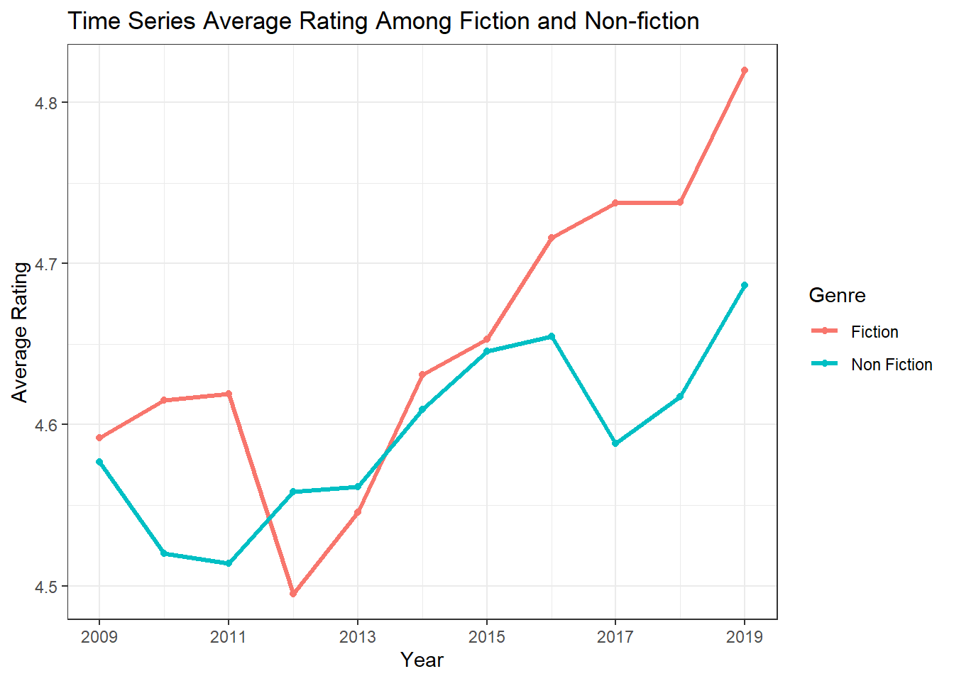
books %>% group_by(Genre, Year) %>%
  summarize(avg_rating = mean(`User Rating`), avg_review = mean(Reviews)) %>%
  ggplot(aes(x = Year, y = avg_review, color = Genre)) +
  geom_line(size = 1.1) +
  geom_point() +
  scale_x_continuous(breaks=seq(2009, 2019, 2)) +
  theme_bw() +
labs(y = "Average Reviews", title = "Time Series Average Reviews Among Fiction and Non-fiction") 
It seems like on average, fictions were more popular than non-fictions throughout this 10-year period except the time in 2012. Also, fictions also attracted more reviews on average than non-fictions besides the year of 2018 when the average reviews of fiction were slightly lower than these of non-fictions.
We can see how pricing being distributed among these bestsellers.
ggplot(books, aes(Price, color = Genre, fill = Genre)) +
geom_histogram(aes(y = ..density..), alpha = 0.6) 
ggplot(books, aes(Price, color = Genre, fill = Genre)) +
geom_histogram(alpha = 0.6) 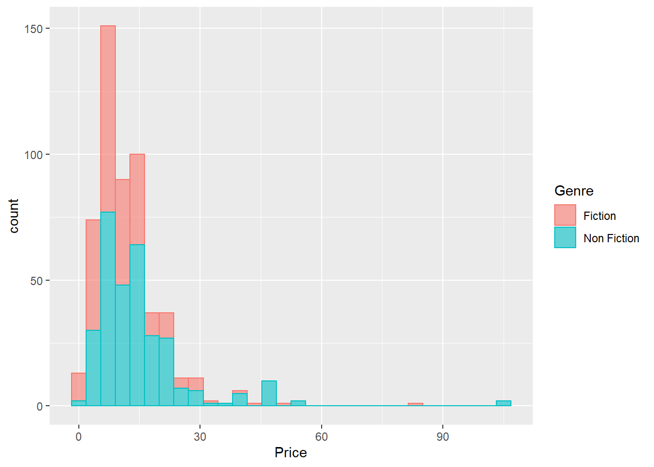
From the plots above, most books (both fiction and non-fiction) are under $30. This makes sense, as the 100-dollar textbooks can never be bestseller!
Machine Learning
Classifying whether a book is fiction or non-fiction based on a number of features is part of the goal of this project. Here we use two algorithm to carry out the task: one algorithm is logistic regression, and the other one is random forest.
Here we split the dataset as 90% training data and 10% testing data and then apply 10-fold corss validation to training data.
Logistic Regression
set.seed(2021)
trainIndex <- createDataPartition(books$Genre_fct, p = .9,
                                  list = FALSE,
                                  times = 1)

booksTrain <- books[ trainIndex,]
booksTest  <- books[-trainIndex,]

train_control <- trainControl(method="cv", number=10)
# train the model
logit_model <- train(Genre_fct ~ `User Rating` + Reviews + Price + Year, data=booksTrain, trControl=train_control, family= "binomial", method="glm")

summary(logit_model)
##
## Call:
## NULL
##
## Deviance Residuals:
## Min 1Q Median 3Q Max
## -2.3901 -0.9630 -0.6921 1.1637 2.4012
##
## Coefficients:
## Estimate Std. Error z value Pr(>|z|)
## (Intercept) 2.042e+02 6.750e+01 3.025 0.00249 **
## `\\`User Rating\\`` 1.202e+00 4.793e-01 2.507 0.01216 *
## Reviews 6.674e-05 1.111e-05 6.005 1.91e-09 ***
## Price -3.831e-02 1.221e-02 -3.137 0.00171 **
## Year -1.044e-01 3.379e-02 -3.090 0.00200 **
## ---
## Signif. codes: 0 '***' 0.001 '**' 0.01 '*' 0.05 '.' 0.1 ' ' 1
##
## (Dispersion parameter for binomial family taken to be 1)
##
## Null deviance: 678.18 on 494 degrees of freedom
## Residual deviance: 609.33 on 490 degrees of freedom
## AIC: 619.33
##
## Number of Fisher Scoring iterations: 4# evaluate the model by using the test data
pred <- predict(logit_model, booksTest, type = "raw")
confusionMatrix(data = booksTest$Genre_fct, pred)## Confusion Matrix and Statistics
##
## Reference
## Prediction 0 1
## 0 25 6
## 1 7 17
##
## Accuracy : 0.7636
## 95% CI : (0.6298, 0.8677)
## No Information Rate : 0.5818
## P-Value [Acc > NIR] : 0.0038
##
## Kappa : 0.5172
##
## Mcnemar's Test P-Value : 1.0000
##
## Sensitivity : 0.7812
## Specificity : 0.7391
## Pos Pred Value : 0.8065
## Neg Pred Value : 0.7083
## Prevalence : 0.5818
## Detection Rate : 0.4545
## Detection Prevalence : 0.5636
## Balanced Accuracy : 0.7602
##
## 'Positive' Class : 0
## Accuracy for logistic regression is around 75%, which is okay. Now we need to see if random forest can do a better job.
Random Forest
set.seed(2021)
rf_grid <-  expand.grid(mtry = c(2,3,4))

model_rf <- train(Genre_fct ~ `User Rating` + Reviews + Price + Year, data=booksTrain, method="rf", trControl = train_control,tuneGrid = rf_grid)

plot(model_rf)
Both mtry = 2 and mtry = 4 have better accuracy than mtry = 3.
rf_pred <- predict(model_rf, booksTest, type = "raw")

confusionMatrix(data = booksTest$Genre_fct, rf_pred)
## Confusion Matrix and Statistics
##
## Reference
## Prediction 0 1
## 0 28 3
## 1 4 20
##
## Accuracy : 0.8727
## 95% CI : (0.7552, 0.9473)
## No Information Rate : 0.5818
## P-Value [Acc > NIR] : 2.878e-06
##
## Kappa : 0.74
##
## Mcnemar's Test P-Value : 1
##
## Sensitivity : 0.8750
## Specificity : 0.8696
## Pos Pred Value : 0.9032
## Neg Pred Value : 0.8333
## Prevalence : 0.5818
## Detection Rate : 0.5091
## Detection Prevalence : 0.5636
## Balanced Accuracy : 0.8723
##
## 'Positive' Class : 0
## As we can see from the output above, random forest is a better model in terms of accuracy and other metrics than logistic regression.
Conclusion
This dataset is a rather clean dataset without having the need to do much preprocessing, and in this analysis we turned it into a binary classification problem where Genre is the response variable and other selected features are predictors. A classical binary-prediction model is logistic regression, which is rather easy to work with but the performance is ususally not as decent as random forest. In this blog post, it is clearly shown that random forest makes better prediction than logistic regression on this very dataset.