Water Potability Data Analysis and Classification
Project Introduction
The dataset is from Kaggle, which indicates that accessing to drinking water is a basic human right. Many places, however, still cannot provide potable water to their residents. In this research project, hopefully, we can use some machine learning algorithms to shed some light on detecting the water quality based on this dataset.
First off, let’s load the appropriate libraries and then explore the dataset a bit.
library(tidyverse)
library(caret)
library(randomForest)
wq <- read_csv("water_potability.csv")
head(wq)## # A tibble: 6 x 10
## ph Hardness Solids Chloramines Sulfate Conductivity Organic_carbon
## <dbl> <dbl> <dbl> <dbl> <dbl> <dbl> <dbl>
## 1 NA 205. 20791. 7.30 369. 564. 10.4
## 2 3.72 129. 18630. 6.64 NA 593. 15.2
## 3 8.10 224. 19910. 9.28 NA 419. 16.9
## 4 8.32 214. 22018. 8.06 357. 363. 18.4
## 5 9.09 181. 17979. 6.55 310. 398. 11.6
## 6 5.58 188. 28749. 7.54 327. 280. 8.40
## # ... with 3 more variables: Trihalomethanes <dbl>, Turbidity <dbl>,
## # Potability <dbl>dim(wq)## [1] 3276 10Data Processing
wq %>% group_by(Potability) %>%
  count()
## # A tibble: 2 x 2
## # Groups: Potability [2]
## Potability n
## <dbl> <int>
## 1 0 1998
## 2 1 1278colSums(is.na(wq))## ph Hardness Solids Chloramines Sulfate
## 491 0 0 0 781
## Conductivity Organic_carbon Trihalomethanes Turbidity Potability
## 0 0 162 0 0wq %>% group_by(Potability) %>%
summarise_all(~sum(is.na(.))) %>%
mutate(Potability, sumNA = rowSums(.[-1]))## # A tibble: 2 x 11
## Potability ph Hardness Solids Chloramines Sulfate Conductivity
## <dbl> <int> <int> <int> <int> <int> <int>
## 1 0 314 0 0 0 488 0
## 2 1 177 0 0 0 293 0
## # ... with 4 more variables: Organic_carbon <int>, Trihalomethanes <int>,
## # Turbidity <int>, sumNA <dbl>We can see that the dataset is slightly imbalanced that there are 700 more water samples not potable than those potable, but there are almost 400 more missing values for not drinkable water than drinkable water. Downsampling could be an option for this project, but let’s see if the results are well in the end without using such a technique.
# Potability column should be a factor rather than a numeric one.
wq$Potability <- factor(wq$Potability)

wq %>% group_by(Potability) %>%
  summarize_all(~mean(., na.rm = TRUE)) %>%
  ungroup() %>%
  pivot_longer(!Potability, names_to = "features", values_to = "mean") %>%
  ggplot(aes(features, mean, fill = Potability)) +
  geom_bar(stat = "identity", position = "dodge") +
  facet_wrap(~features, scales = "free")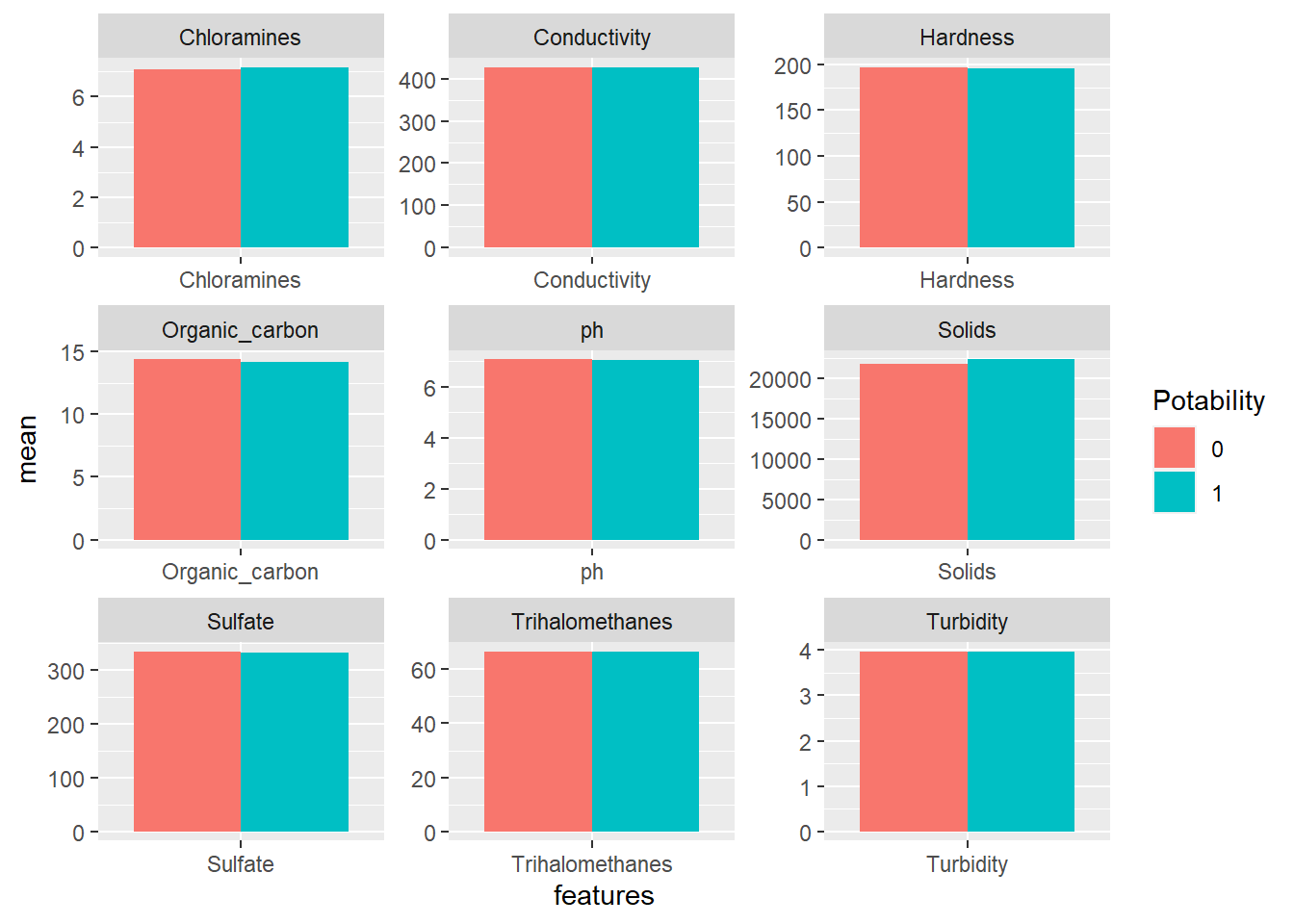
Based on the mean of each feature, both types of water are kind of similar. Maybe mean is not a good indicator for comparing them. Let’s use minimum instead.
wq %>% group_by(Potability) %>%
  summarize_all(~min(., na.rm = TRUE)) %>%
  ungroup() %>%
  pivot_longer(!Potability, names_to = "features", values_to = "min") %>%
  ggplot(aes(features, min, fill = Potability)) +
  geom_bar(stat = "identity", position = "dodge") +
  facet_wrap(~features, scales = "free")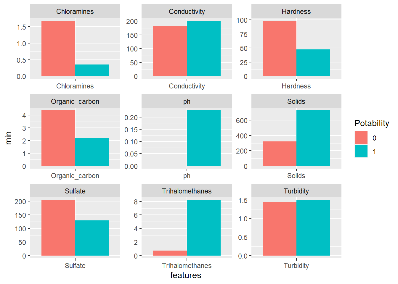
Now we can see some salient differences among the features between the two types of water. The minimum values of Chloramines, Hardness, Organic_carbon and Sulfate are much higher in non-potable water than in potabile water.
PCA
Since this is a binary-classification problem with 9 potential features, using PCA in the first place to lower dimensions and then give some plots would help us understand the problem better.
# Applying PCA and data viz
x1 <- preProcess(wq %>% select(-Potability), method = "pca", pcaComp = 2)
x2 <- predict(x1, wq %>% select(-Potability))
x2 %>% mutate(
  Potability = wq$Potability
) %>%
  ggplot(aes(PC1, PC2, color = Potability)) +
  geom_point()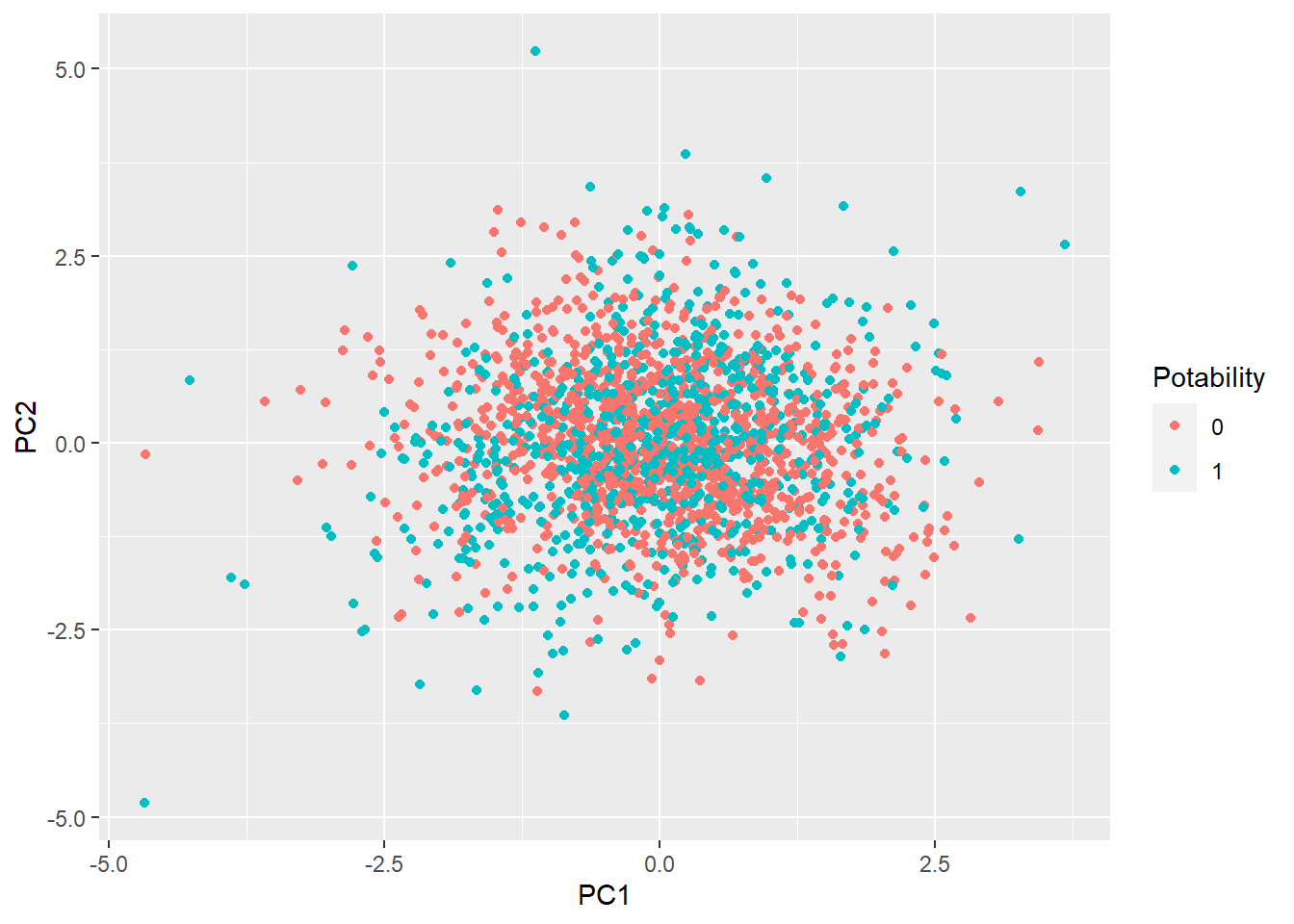
Based on the plot above, it seems like there is no an obvious pattern to differentiate the classes.
Now, we use three machine learning algorithms on this very dataset and see how they perform. First off, it is intuitive to use logistic regression, as it is a classical binary-classification problem.
Logistic Regression
wq_filter <- drop_na(wq)

set.seed(2021)
trainIndex <- createDataPartition(wq_filter$Potability, p = .7,
                                  list = FALSE,
                                  times = 1)

wq_filterTrain <- wq_filter[ trainIndex,]
wq_filterTest  <- wq_filter[-trainIndex,]

train_control <- trainControl(method="cv", number=10)

# train the model
logit_model <- train(Potability ~ ., data= wq_filterTrain, trControl=train_control, family= "binomial", method="glm")

summary(logit_model)
##
## Call:
## NULL
##
## Deviance Residuals:
## Min 1Q Median 3Q Max
## -1.2345 -1.0220 -0.9489 1.3200 1.6060
##
## Coefficients:
## Estimate Std. Error z value Pr(>|z|)
## (Intercept) -1.296e+00 9.076e-01 -1.428 0.1532
## ph 3.891e-02 3.578e-02 1.088 0.2767
## Hardness -6.525e-04 1.734e-03 -0.376 0.7066
## Solids 1.102e-05 6.483e-06 1.700 0.0891 .
## Chloramines 4.319e-02 3.566e-02 1.211 0.2258
## Sulfate 3.553e-04 1.366e-03 0.260 0.7948
## Conductivity -7.937e-04 6.736e-04 -1.178 0.2387
## Organic_carbon 1.419e-03 1.646e-02 0.086 0.9313
## Trihalomethanes -1.025e-04 3.448e-03 -0.030 0.9763
## Turbidity 1.029e-01 7.083e-02 1.453 0.1463
## ---
## Signif. codes: 0 '***' 0.001 '**' 0.01 '*' 0.05 '.' 0.1 ' ' 1
##
## (Dispersion parameter for binomial family taken to be 1)
##
## Null deviance: 1899.0 on 1407 degrees of freedom
## Residual deviance: 1890.4 on 1398 degrees of freedom
## AIC: 1910.4
##
## Number of Fisher Scoring iterations: 4pred <- predict(logit_model, wq_filterTest, type = "raw")
confusionMatrix(data = wq_filterTest$Potability, pred)## Confusion Matrix and Statistics
##
## Reference
## Prediction 0 1
## 0 358 2
## 1 238 5
##
## Accuracy : 0.602
## 95% CI : (0.5617, 0.6413)
## No Information Rate : 0.9884
## P-Value [Acc > NIR] : 1
##
## Kappa : 0.0178
##
## Mcnemar's Test P-Value : <2e-16
##
## Sensitivity : 0.60067
## Specificity : 0.71429
## Pos Pred Value : 0.99444
## Neg Pred Value : 0.02058
## Prevalence : 0.98839
## Detection Rate : 0.59370
## Detection Prevalence : 0.59701
## Balanced Accuracy : 0.65748
##
## 'Positive' Class : 0
## The logistic regression has a medicore performance on the test dataset, and the false positive rate is surprisingly high, meaning many water samples that are not drinkable but predicted drinkable.
Support Vector Machine
svm_radial <- train(Potability ~ ., data= wq_filterTrain, trControl=train_control,  method = "svmRadial", preProcess = c("center","scale"), tuneLength = 10)
#"svmRadial" "svmLinear"
pred_svm_radial <- predict(svm_radial, wq_filterTest)

confusionMatrix(data = wq_filterTest$Potability, pred_svm_radial)
## Confusion Matrix and Statistics
##
## Reference
## Prediction 0 1
## 0 332 28
## 1 154 89
##
## Accuracy : 0.6982
## 95% CI : (0.6598, 0.7346)
## No Information Rate : 0.806
## P-Value [Acc > NIR] : 1
##
## Kappa : 0.315
##
## Mcnemar's Test P-Value : <2e-16
##
## Sensitivity : 0.6831
## Specificity : 0.7607
## Pos Pred Value : 0.9222
## Neg Pred Value : 0.3663
## Prevalence : 0.8060
## Detection Rate : 0.5506
## Detection Prevalence : 0.5970
## Balanced Accuracy : 0.7219
##
## 'Positive' Class : 0
## Random Forest
set.seed(2021)
rf_grid <-  expand.grid(mtry = seq(2,9))

model_rf <- train(Potability ~ ., data= wq_filterTrain, trControl=train_control, method="rf", tuneGrid = rf_grid)

plot(model_rf)
rf_pred <- predict(model_rf, wq_filterTest, type = "raw")

confusionMatrix(data = wq_filterTest$Potability, rf_pred)
## Confusion Matrix and Statistics
##
## Reference
## Prediction 0 1
## 0 309 51
## 1 132 111
##
## Accuracy : 0.6965
## 95% CI : (0.6581, 0.733)
## No Information Rate : 0.7313
## P-Value [Acc > NIR] : 0.9748
##
## Kappa : 0.3332
##
## Mcnemar's Test P-Value : 3.344e-09
##
## Sensitivity : 0.7007
## Specificity : 0.6852
## Pos Pred Value : 0.8583
## Neg Pred Value : 0.4568
## Prevalence : 0.7313
## Detection Rate : 0.5124
## Detection Prevalence : 0.5970
## Balanced Accuracy : 0.6929
##
## 'Positive' Class : 0
## Variable importance is worthwhile to look at and see if we need to select a subset of features.
gbmImp <- varImp(model_rf, scale = FALSE)
plot(gbmImp)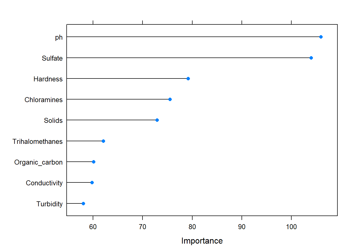
Let’s try to choose ph, Sulfate, Hardness and Chloramines as features to train and see if the random forest model would be better.
set.seed(2021)

rf_grid_subset <-  expand.grid(mtry = seq(2,4))

model_rf_subset <- train(Potability ~ ph + Sulfate + Hardness + Chloramines, data= wq_filterTrain, trControl=train_control, method="rf", tuneGrid = rf_grid_subset)

plot(model_rf_subset)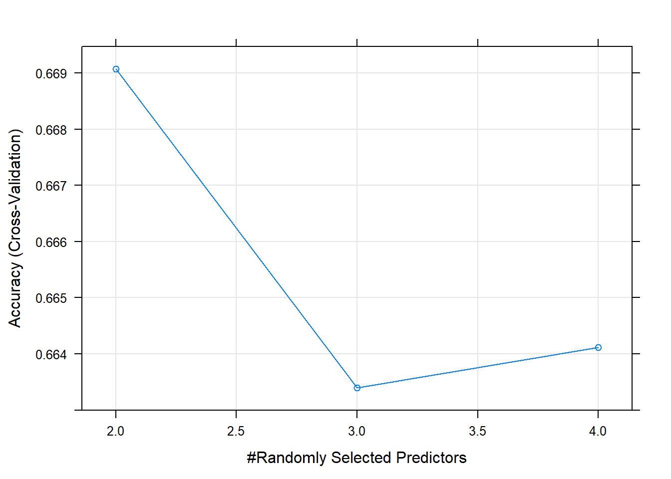
rf_pred_subset <- predict(model_rf_subset, wq_filterTest, type = "raw")

confusionMatrix(data = wq_filterTest$Potability, rf_pred_subset)
## Confusion Matrix and Statistics
##
## Reference
## Prediction 0 1
## 0 289 71
## 1 124 119
##
## Accuracy : 0.6766
## 95% CI : (0.6377, 0.7138)
## No Information Rate : 0.6849
## P-Value [Acc > NIR] : 0.6865982
##
## Kappa : 0.3032
##
## Mcnemar's Test P-Value : 0.0001962
##
## Sensitivity : 0.6998
## Specificity : 0.6263
## Pos Pred Value : 0.8028
## Neg Pred Value : 0.4897
## Prevalence : 0.6849
## Detection Rate : 0.4793
## Detection Prevalence : 0.5970
## Balanced Accuracy : 0.6630
##
## 'Positive' Class : 0
## It turned out that the subset of features being fed into the random forest model gave us some slightly worse results than the random forest model with the full set of features.
Conclusion
In terms of prediction accuracy, none of the algorithms we tried have stood out, and all of the accuracies are below 70%. Random forest seems like to perform the best, but it is only slightly better than svm with the radial kernel. In order to improve the performance, there are two parts we can do. One is to continue to use the current algorithms, but parameters should be tuned further. The other one is to use a more complicated machine learning algorithm such as neural network to train and test the dataset.