Changepoint Detection And Data Visualization On Facebook Stock Dataset
In this project, we analyze Facebook stock dataset found on Kaggle, which is time-series related. There is a wonderful R package lubridate, which has made any work dealing with date handy and less miserable. Besides few time-series data visualizations we will make, changepoint detection will also be carried out on a number of key indexes of the stock.
Data Introduction
After loading the related libraries, the dataset fb.csv is loaded and as always, using janitor::clean_names to clean up the rownames so that they are easy to reference later.
library(tidyverse)
library(lubridate)
library(scales)
library(changepoint)
fb <- read_csv("fb.csv")
fb <- janitor::clean_names(fb)
head(fb)## # A tibble: 6 x 7
## date open high low close adj_close volume
## <date> <dbl> <dbl> <dbl> <dbl> <dbl> <dbl>
## 1 2012-05-18 42.0 45 38 38.2 38.2 573576400
## 2 2012-05-21 36.5 36.7 33 34.0 34.0 168192700
## 3 2012-05-22 32.6 33.6 30.9 31 31 101786600
## 4 2012-05-23 31.4 32.5 31.4 32 32 73600000
## 5 2012-05-24 33.0 33.2 31.8 33.0 33.0 50237200
## 6 2012-05-25 32.9 33.0 31.1 31.9 31.9 37149800dim(fb)## [1] 2320 7tail(fb)## # A tibble: 6 x 7
## date open high low close adj_close volume
## <date> <dbl> <dbl> <dbl> <dbl> <dbl> <dbl>
## 1 2021-07-30 354 361. 353. 356. 356. 15966700
## 2 2021-08-02 358. 359. 351. 352. 352. 13180400
## 3 2021-08-03 353. 354. 348. 351. 351. 12393000
## 4 2021-08-04 352. 360. 352. 359. 359. 14180600
## 5 2021-08-05 360. 364. 357. 363. 363. 10247200
## 6 2021-08-06 361. 365. 361. 364. 364. 8918100As shown from part of the output above, Facebook went to public on May 18th 2012 and the dataset ends on Auguest 6th 2021.
Now let’s use skim() to give an overview of the dataset to evaluate the statistics of each column and if each one has any missing values.
skimr::skim(fb)| Name | fb |
| Number of rows | 2320 |
| Number of columns | 7 |
| _______________________ | |
| Column type frequency: | |
| Date | 1 |
| numeric | 6 |
| ________________________ | |
| Group variables | None |
Variable type: Date
| skim_variable | n_missing | complete_rate | min | max | median | n_unique |
|---|---|---|---|---|---|---|
| date | 0 | 1 | 2012-05-18 | 2021-08-06 | 2016-12-27 | 2320 |
Variable type: numeric
| skim_variable | n_missing | complete_rate | mean | sd | p0 | p25 | p50 | p75 | p100 | hist |
|---|---|---|---|---|---|---|---|---|---|---|
| open | 0 | 1 | 135.84 | 79.99 | 18.08 | 74.49 | 129.08 | 183.50 | 374.56 | ▇▆▆▂▁ |
| high | 0 | 1 | 137.44 | 80.96 | 18.27 | 75.23 | 129.94 | 185.35 | 377.55 | ▇▆▆▂▁ |
| low | 0 | 1 | 134.23 | 79.09 | 17.55 | 73.72 | 128.14 | 181.54 | 368.22 | ▇▆▆▂▁ |
| close | 0 | 1 | 135.89 | 80.07 | 17.73 | 74.58 | 129.02 | 183.59 | 373.28 | ▇▆▆▂▁ |
| adj_close | 0 | 1 | 135.89 | 80.07 | 17.73 | 74.58 | 129.02 | 183.59 | 373.28 | ▇▆▆▂▁ |
| volume | 0 | 1 | 31252504.78 | 27905827.98 | 5913100.00 | 15865775.00 | 22557950.00 | 36194225.00 | 573576400.00 | ▇▁▁▁▁ |
Data Processing
This is a rather clean dataset without any missing value and analysis is good to go. Therefore, it is relatively easy to process data. Please also note if there were any missing value in any column, it would be much easier to impute the respective value given the fact that all stock information is public and easily accessible.
When there is a date column presented in the dataset, sometimes it is handy to create extra columns to single out year and month.
fb <- fb %>%
  mutate(year = year(date),
         month = month(date))
Data Visualization
Not plotting the time-series open index and close index throughtout the entire time span given by the dataset. Also, a loess curve is genereated to fit the trends. Both plots show that there is an upward trend for the stock pricing.
ggplot(fb, aes(date, open)) +
  geom_line()+
  geom_point() +
  labs(x = "Year", y = "Open Index", title = "Facebook Open Index") +
  scale_x_date(labels = date_format("%Y"), breaks = "1 year")+
  geom_smooth(model = "loess", color = "green")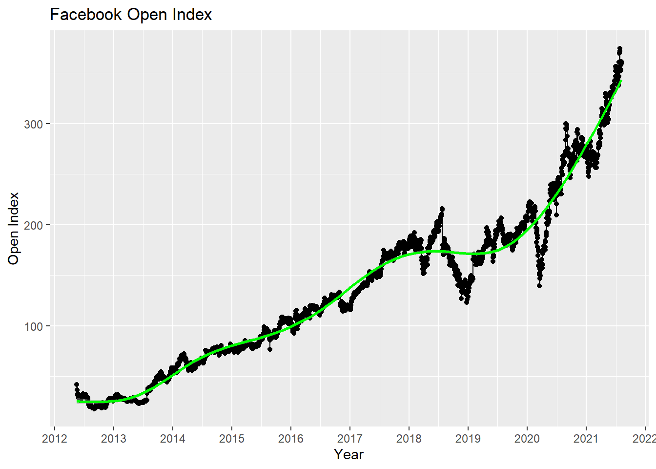
ggplot(fb, aes(date, close)) +
  geom_line()+
  geom_point() +
  labs(x = "Year", y = "Close Index", title = "Facebook Close Index") +
  scale_x_date(labels = date_format("%Y"), breaks = "1 year") +
  geom_smooth(model = "loess", color = "green")
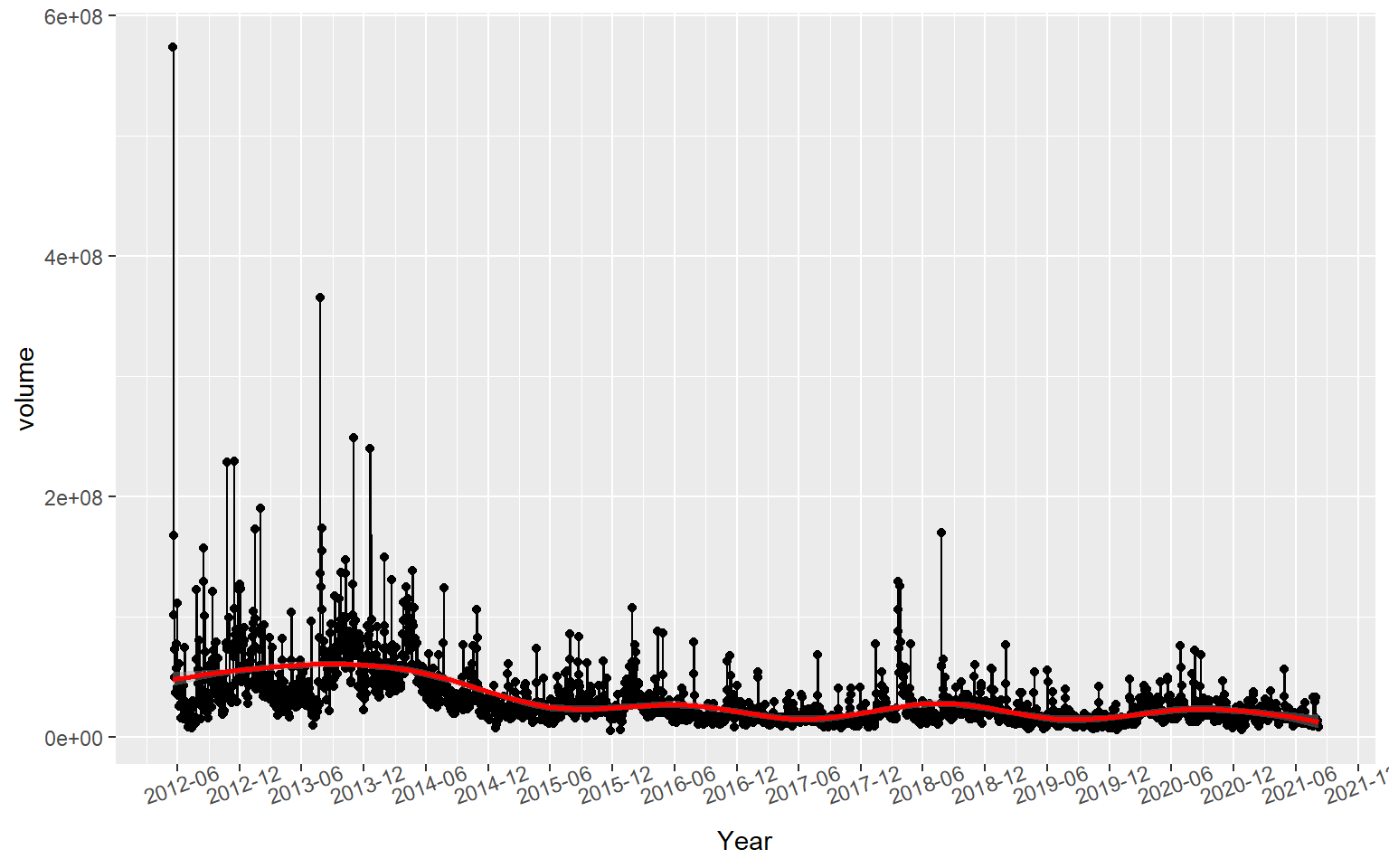
In terms of volume, its time series plot needs to take log transformation, since there were a number of outliers that were significant and they would make the majority of data points close to x axis. A loess curve also fits the data.
ggplot(fb, aes(date, volume)) +
  geom_line()+
  geom_point() +
  labs(x = "Year") +
  scale_x_date(labels = date_format("%Y-%m"), breaks = "6 months") +
  geom_smooth(model = "loess", color = "red") +
  theme(
    axis.text.x = element_text(angle = 20)
  )
ggplot(fb, aes(date, volume)) +
  geom_line()+
  geom_point() +
  labs(x = "Year") +
  scale_x_date(labels = date_format("%Y-%m"), breaks = "6 months") +
  scale_y_log10() +
  geom_smooth(model = "loess", color = "red") +
  theme(
    axis.text.x = element_text(angle = 20)
  )
It is worth noting that although the stock pricing grew significantly year by year, but the volume did not. Although it experienced some sinuous trends, it had a somewhat downward trend based on the log-scale loess curve.
fb %>%
  group_by(year, month) %>%
  summarize(avg = mean(open)) %>%
  ggplot(aes(month, avg, color = year)) +
  geom_line() +
  geom_point() +
  scale_x_continuous(labels = seq(1,12,2), breaks = seq(1,12,2)) +
  facet_wrap(~year) +
  theme_bw() +
  theme(
    legend.position = "none",
    strip.text = element_text(size = 13),
    axis.ticks = element_blank()
  ) +
  labs(x = "Month", y = "Mean Open Price", title = "Year-Wise Mean Open Pricing")
fb %>%
  group_by(year, month) %>%
  summarize(avg = mean(volume)) %>%
  ggplot(aes(month, avg, color = year)) +
  geom_line() +
  geom_point() +
  scale_x_continuous(labels = seq(1,12,2), breaks = seq(1,12,2)) +
  scale_y_log10() +
  facet_wrap(~year) +
  theme_bw() +
  theme(
    legend.position = "none",
    strip.text = element_text(size = 13),
    axis.ticks = element_blank()
  ) +
  labs(x = "Month", y = "Log-10-Scale Mean Volume", title = "Year-Wise Log-Scale Mean Volume")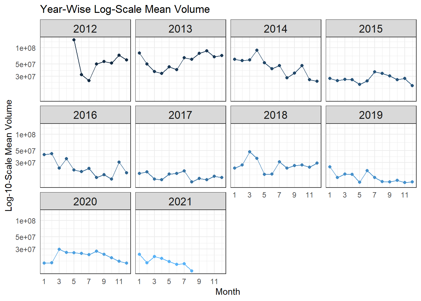
Changepoint Detection
There are a number of changepoint detection packages built in R (changepoint, bcp, ecp, etc.). In this section, we are going to use changepoint package to detect changepoints. Moreover, cpt.meanvar() is the primary function we use, unlike cpt.mean() and cpt.var(), it respects both mean and variance of data when detecting changepoints. The method parameter is set to be PELT, which stands for Pruned Exact Linear Time, opposite of AMOC or At Most One Changepoint. If we deem that data has more than more changepoint, the default method would always be PELT.
One thing we should note is that changepoint detection is a subjective concept. When looking at the same time-series data, different people have different opinions on where changepoints should be drawn. Since all changepoint algorithms are designed by human beings, whatever outputs are, they will also be subjective.
cpt_volume <- cpt.meanvar(fb$volume, method = "PELT")
log_cpt_volume <- cpt.meanvar(log10(fb$volume), method = "PELT")
cpt_open <- cpt.meanvar(fb$open, method = "PELT")
plot(cpt_volume, xlab = "Day(s) Since Going Public", ylab = "Volume", main = "Changepoints On FB Volume")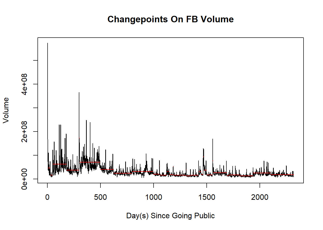
plot(log_cpt_volume, xlab = "Day(s) Since Going Public", ylab = "Log-Scale Volume", main = "Log-Scale Changepoints On FB Volume")
plot(cpt_open, xlab = "Day(s) Since Going Public", ylab = "Open Price", main = "Changepoints On FB Open Price")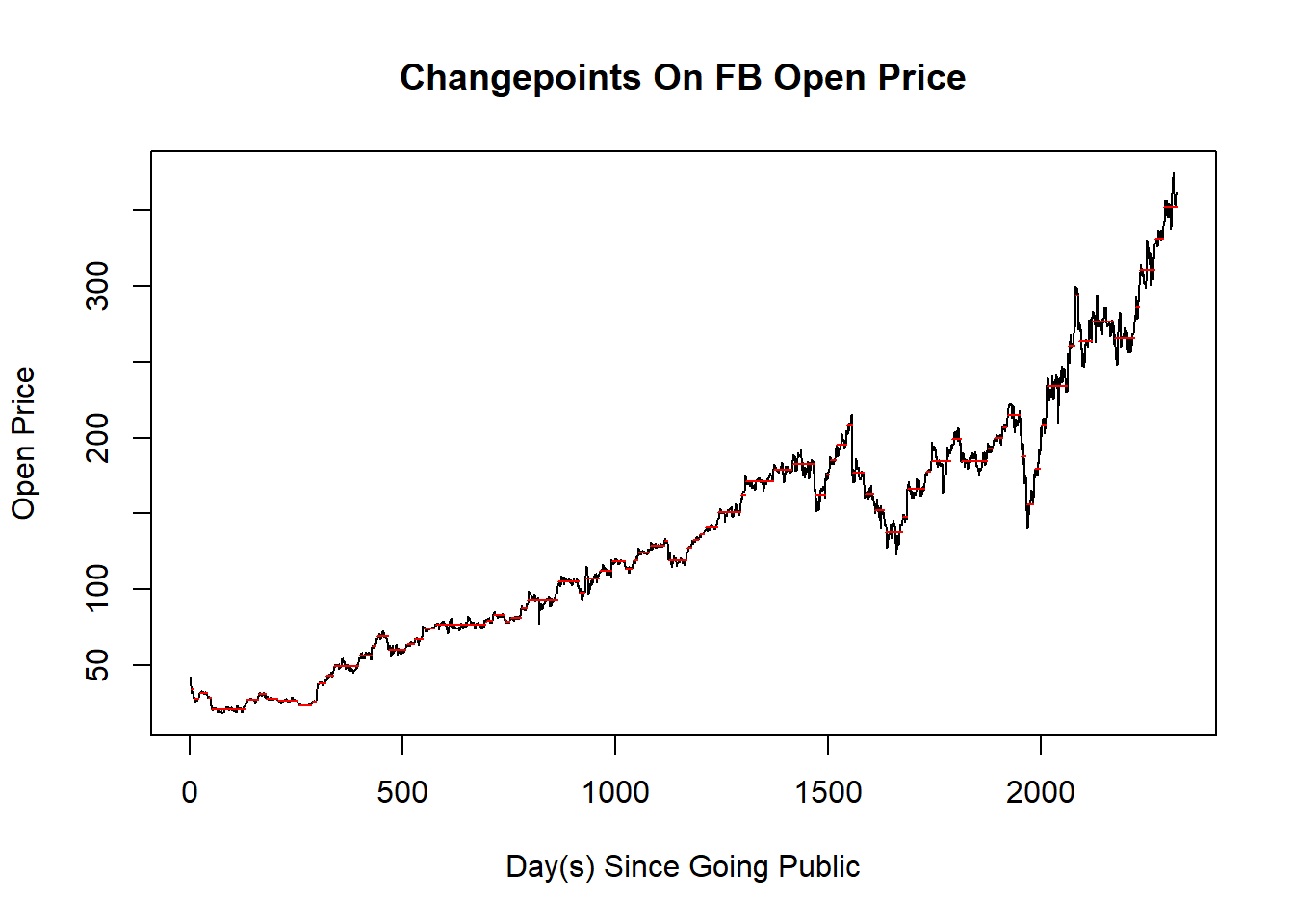
avg_open <- fb %>%
  group_by(year, month) %>%
  summarize(avg = mean(open))
avg_open_ts <- ts(avg_open$avg, frequency = 12, start= c(2012,5), end= c(2021, 7))

avg_volume <- fb %>%
  group_by(year, month) %>%
  summarize(avg = mean(volume))

avg_volume_ts <- ts(avg_volume$avg, frequency = 12, start= c(2012,5), end= c(2021, 7))

plot(cpt.meanvar(avg_open_ts, method = "PELT"), xlab = "Year", ylab = "Mean Open Index", main = "Changepoints On The Mean FB Open Index")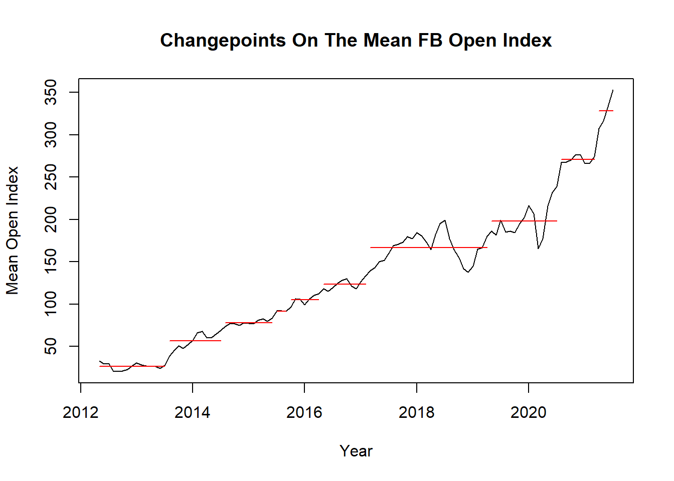
plot(cpt.meanvar(avg_volume_ts, method = "PELT"), xlab = "Year", ylab = "Mean Volume", main = "Changepoints On The Mean FB Volume")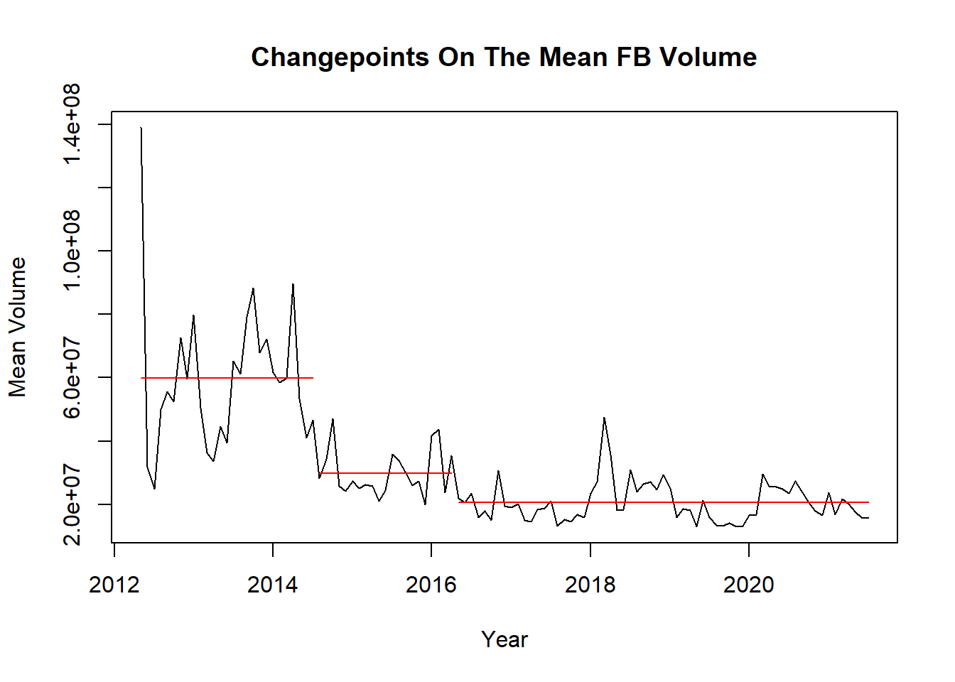
cpts(cpt_volume)## [1] 2 25 47 178 295 301 495 621 794 994 1053 1056 1122 1143 1183
## [16] 1185 1304 1308 1346 1422 1445 1466 1473 1498 1554 1559 1689 1706 1808 1935
## [31] 2100cpts(log_cpt_volume)## [1] 28 47 185 295 496 621 776 1000 1002 1186 1422 1445 1465 1498 1554
## [16] 1560 1689 1952 2135What is interesting is that when using log10() on the original data, the changepoint detections vary based on the output above.
cpts(cpt.meanvar(avg_open_ts, method = "PELT"))## [1] 15 27 38 41 48 58 84 99 107cpts(cpt.meanvar(avg_volume_ts, method = "PELT"))## [1] 27 48Only index = 27 and index = 48 are in both outputs.
Conclusion
In this project, we analyzed Facebook stock dataset based on a number of key factors with visualizations that include loess curve, and changepoint detection is also added to check if the detection is consistent among different data points. Overall, there is an upward trend based on both open and close pricing, which indicates Facebook has been a growing company since it went public, yet the volume turns out be going down. Also, changepoint detection is not consistent not only when applying this real-world dataset but it is highly subjective in general.
This project can be extended to time-series prediction to estimate how Facebook stock pricing will be changing in the future. If anybody is interested in doing so, this current report may have already shed some light in this respect.