US Fast Food Chain Exploratory Data Analysis And Data Quality Check
Fast food chains are ubiquitous. In this Kaggle dataset, it has records of 10000 fast food restaurants here in the U.S. across 50 states and Washington D.C. In this project, we would like to explore this dataset to see which fast food chains are among the most popular ones nationwide and each statewide. Also, data quality is rather important, and after exploring the dataset, we would like to check the quality of this dataset and use common sense to evaluate the data quality.
To begin with, let’s load the libraries. Since part of the analysis will be about the U.S. states, it will be useful to use facet_geo() from geofacet library.
library(tidyverse)
library(geofacet)
Dataset Exploration
ff <- read_csv("FastFoodRestaurants.csv")
head(ff)
## # A tibble: 6 x 10
## address city country keys latitude longitude name postalCode province
## <chr> <chr> <chr> <chr> <dbl> <dbl> <chr> <chr> <chr>
## 1 324 Mai~ Massena US us/ny/m~ 44.9 -74.9 McDo~ 13662 NY
## 2 530 Cli~ Washin~ US us/oh/w~ 39.5 -83.4 Wend~ 43160 OH
## 3 408 Mar~ Maysvi~ US us/ky/m~ 38.6 -83.8 Fris~ 41056 KY
## 4 6098 St~ Massena US us/ny/m~ 45.0 -74.8 McDo~ 13662 NY
## 5 139 Col~ Athens US us/oh/a~ 39.4 -82.1 OMG!~ 45701 OH
## 6 4182 To~ Hamilt~ US us/oh/h~ 39.4 -84.5 Domi~ 45011 OH
## # ... with 1 more variable: websites <chr>dim(ff)## [1] 10000 10When glancing the dataset, one thing we find out a bit strange is some column names. name column is fast food chain names, province is each state. Without causing any confusion later, it is better to rename these two columns.
ff <- ff %>%
  rename(chain_name = name,
state = province)skimr::skim(ff)| Name | ff |
| Number of rows | 10000 |
| Number of columns | 10 |
| _______________________ | |
| Column type frequency: | |
| character | 8 |
| numeric | 2 |
| ________________________ | |
| Group variables | None |
Variable type: character
| skim_variable | n_missing | complete_rate | min | max | empty | n_unique | whitespace |
|---|---|---|---|---|---|---|---|
| address | 0 | 1.00 | 5 | 60 | 0 | 9934 | 0 |
| city | 0 | 1.00 | 3 | 23 | 0 | 2775 | 0 |
| country | 0 | 1.00 | 2 | 2 | 0 | 1 | 0 |
| keys | 0 | 1.00 | 26 | 109 | 0 | 10000 | 0 |
| chain_name | 0 | 1.00 | 3 | 51 | 0 | 548 | 0 |
| postalCode | 0 | 1.00 | 4 | 10 | 0 | 5289 | 0 |
| state | 0 | 1.00 | 2 | 7 | 0 | 52 | 0 |
| websites | 465 | 0.95 | 13 | 1087 | 0 | 3821 | 0 |
Variable type: numeric
| skim_variable | n_missing | complete_rate | mean | sd | p0 | p25 | p50 | p75 | p100 | hist |
|---|---|---|---|---|---|---|---|---|---|---|
| latitude | 0 | 1 | 37.55 | 5.05 | -6.24 | 34.03 | 38.30 | 41.12 | 64.84 | ▁▁▆▇▁ |
| longitude | 0 | 1 | -91.06 | 18.56 | -159.38 | -97.41 | -87.66 | -81.46 | 123.01 | ▂▇▁▁▁ |
There is Co Spgs in the state column. After looking it closely, it should be CO and we use case_when function to change it while preserving other values.
unique(ff$state)## [1] "NY" "OH" "KY" "SC" "AR" "OK" "IN"
## [8] "NC" "TN" "TX" "LA" "KS" "ND" "UT"
## [15] "GA" "NM" "OR" "HI" "VT" "MI" "MO"
## [22] "WI" "WA" "MS" "NE" "ME" "MN" "AL"
## [29] "IA" "WV" "AZ" "SD" "WY" "IL" "VA"
## [36] "FL" "CA" "MT" "ID" "PA" "RI" "NV"
## [43] "NJ" "MA" "MD" "CO" "NH" "CT" "AK"
## [50] "DE" "DC" "Co Spgs"ff <- ff %>%
mutate(state = case_when(state == "Co Spgs" ~ "CO",
TRUE ~ as.character(state)))
unique(ff$state)## [1] "NY" "OH" "KY" "SC" "AR" "OK" "IN" "NC" "TN" "TX" "LA" "KS" "ND" "UT" "GA"
## [16] "NM" "OR" "HI" "VT" "MI" "MO" "WI" "WA" "MS" "NE" "ME" "MN" "AL" "IA" "WV"
## [31] "AZ" "SD" "WY" "IL" "VA" "FL" "CA" "MT" "ID" "PA" "RI" "NV" "NJ" "MA" "MD"
## [46] "CO" "NH" "CT" "AK" "DE" "DC"It is interesting to see which state has the largest number of fast food chains.
ff %>%
  count(state, sort = TRUE) %>%
  mutate(state = fct_reorder(state, n)) %>%
  ggplot(aes(state, n, fill = n)) +
  geom_col() +
  coord_flip() +
  labs(x = "State", y = "Fast Food Chain Count", title = "Fast Food Chain Count In Each State") +
  theme_bw() +
  theme(
    legend.position = "none",
    axis.text = element_text(size = 11),
    axis.title = element_text(size = 15),
    plot.title = element_text(size = 18)
  )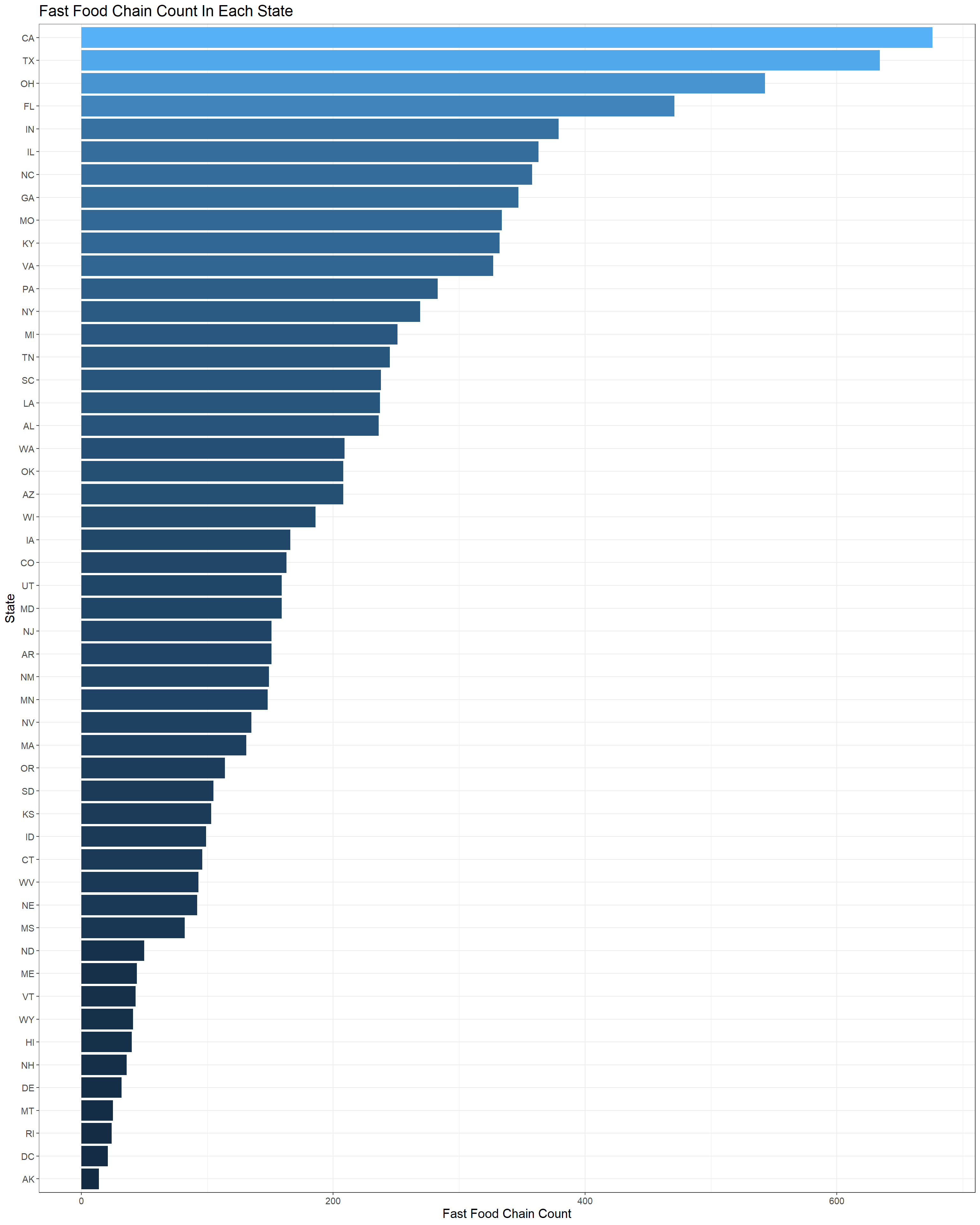
The above bar chart is not accurate in a way that some would argue the reason why California has the largest number of fast food chains is that the state is one of the largest and much more populated than some tiny states. Therefore, it is more reasonable to count fast food chains per 100 thousands of residents in each state.
length(unique(ff$chain_name))## [1] 548Since there are 548 unique chains, it is impossible to include all of them in one plot, and there is no such a need to do so. fct_lump() is such a wonderful function that lumps many chains into Other while keeping the top ones based on users’ input, and fct_reorder() works well with geom_col() to rearrange the bar chart from the largest one down to the smallest one, or vice versa.
Here we give the top 20 fast food chains in the U.S.
ff %>%
  count(chain_name, sort = TRUE) %>%
  mutate(chain_name = fct_lump(chain_name, n = 20, w = n),
         chain_name = fct_reorder(chain_name, n)) %>%
  ggplot(aes(chain_name, n, fill = n)) +
  geom_col() +
  coord_flip() +
  labs(x = "", y = "Fast Food Chain Count", title = "US Top 20 Fast Food Chain Count Overview") +
  theme_bw() +
  theme(
    legend.position = "none",
    axis.text = element_text(size = 11),
    axis.title = element_text(size = 15),
    plot.title = element_text(size = 18)
  )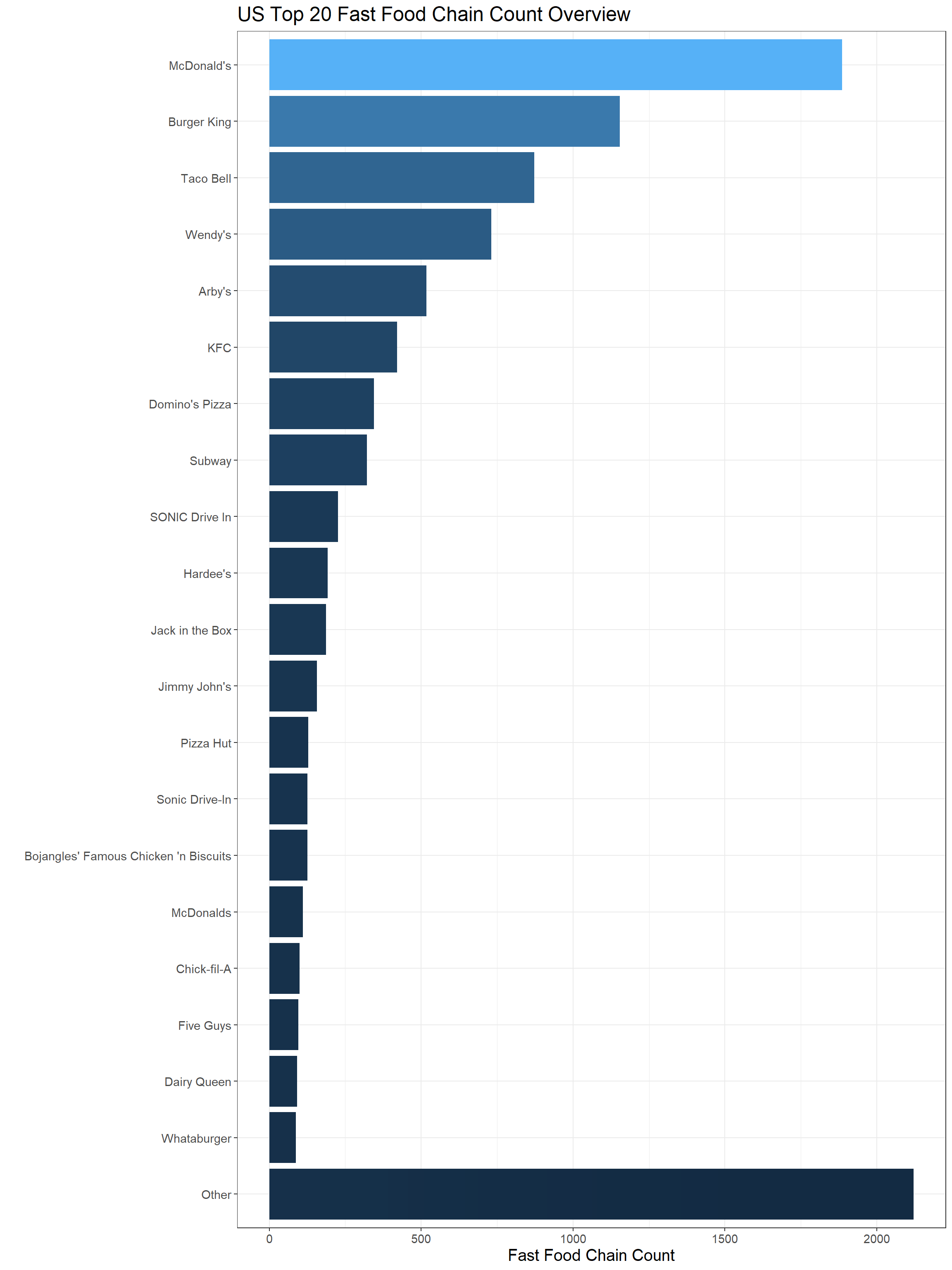
Some data processing after we found out that McDonald's has various spellings, such as Mcdonald's and McDonalds etc.
ff %>%
  filter(chain_name == "McDonalds")
## # A tibble: 111 x 10
## address city country keys latitude longitude chain_name postalCode state
## <chr> <chr> <chr> <chr> <dbl> <dbl> <chr> <chr> <chr>
## 1 8401 Ga~ El Pa~ US us/tx~ 31.8 -106. McDonalds 79925 TX
## 2 3898 Cl~ Dalton US us/ga~ 34.9 -84.9 McDonalds 30721 GA
## 3 4204 Mi~ Sandu~ US us/oh~ 41.4 -82.7 McDonalds 44870 OH
## 4 2984 Up~ Sidney US us/ne~ 41.1 -103. McDonalds 69162 NE
## 5 905 W C~ Swans~ US us/nc~ 34.7 -77.1 McDonalds 28584 NC
## 6 441 Cra~ Buffa~ US us/tx~ 31.5 -96.1 McDonalds 75831 TX
## 7 327 S C~ Carls~ US us/nm~ 32.4 -104. McDonalds 88220 NM
## 8 2050 N ~ Bourb~ US us/il~ 41.2 -87.9 McDonalds 60914 IL
## 9 2883 S ~ Fort ~ US us/sc~ 35.1 -81.0 McDonalds 29708 SC
## 10 2750 Fr~ Owens~ US us/ky~ 37.7 -87.1 McDonalds 42301 KY
## # ... with 101 more rows, and 1 more variable: websites <chr>ff <- ff %>%
mutate(chain_name = case_when(chain_name == "McDonalds" ~ "McDonald's",
chain_name == "Mcdonald's" ~ "McDonald's",
TRUE ~ as.character(chain_name)))ff %>%
count(chain_name, sort = TRUE) %>%
mutate(chain_name = fct_lump(chain_name, n = 20, w = n),
chain_name = fct_reorder(chain_name, n)) %>%
ggplot(aes(chain_name, n, fill = n)) +
geom_col() +
coord_flip() +
labs(x = "", y = "Fast Food Chain Count", title = "US Top 20 Fast Food Chain Count Overview") +
theme_bw() +
theme(
legend.position = "none",
axis.text = element_text(size = 11),
axis.title = element_text(size = 15),
plot.title = element_text(size = 18)
)
It is interesting to use facet_geo() to visualize 5 most popular fast food chains in each state.
ff %>%
  count(state, chain_name, sort = TRUE) %>%
  mutate(chain_name = fct_lump(chain_name, n = 5, w = n),
         chain_name = fct_reorder(chain_name, n)) %>%
  ggplot(aes(chain_name, n, fill = chain_name)) +
  geom_col() +
  coord_flip() +
  facet_geo(~state, scales = "free_x") +
  theme_bw() +
  theme(
    strip.text = element_text(size = 18),
    axis.text = element_text(size = 14),
    legend.position = "none",
    axis.title.y = element_blank(),
    axis.title.x = element_text(size = 20),
    plot.title = element_text(size = 30)
  ) +
  labs(y = "Fast Food Resturant Count", title = "Top 5 Fast Food Resturants In Each State")
Data Quality Check
Let’s look at top 20 fast food chains in Ohio first. There are only 3 Chick-fil-A in the entire state based on the output below. How is this possible?
ff %>%
  filter(state == "OH") %>%
  count(chain_name, sort = TRUE) %>%
  top_n(20)
## # A tibble: 25 x 2
## chain_name n
## <chr> <int>
## 1 McDonald's 114
## 2 Burger King 72
## 3 Wendy's 69
## 4 Taco Bell 53
## 5 Arby's 48
## 6 KFC 24
## 7 White Castle 22
## 8 Jimmy John's 14
## 9 Gold Star Chili 8
## 10 Boston Market 7
## # ... with 15 more rowsff %>%
filter(state == "OH") %>%
count(chain_name, sort = TRUE) %>%
filter(chain_name == "Chick-fil-A")## # A tibble: 1 x 2
## chain_name n
## <chr> <int>
## 1 Chick-fil-A 3Also, the entire country only has one Starbucks, which is in Ohio.
ff %>%
  filter(str_detect(str_to_lower(chain_name), "starbucks"))
## # A tibble: 1 x 10
## address city country keys latitude longitude chain_name postalCode state
## <chr> <chr> <chr> <chr> <dbl> <dbl> <chr> <chr> <chr>
## 1 5555 You~ Niles US us/oh/~ 41.2 -80.8 Starbucks 44446 OH
## # ... with 1 more variable: websites <chr>After carrying out some basic quality checks, it is not difficult for us to see there is some serious issue related to the quality of this dataset. The more accurate interpretation of it would be that the dataset only contains 10000 fast food restaurants in the U.S., but that is far from the complete picture of the true distribution of fast food restaurants in America. It is always important to have an eye on data quality, especially when data sourcing is not something that might have been conducted in a serious manner. Using such a dataset would output misleading results, however solid our approach is.
Conclusion
In this project, we used a fast food dataset and saw that McDonald’s is the most popular fast food chain in America. And regarding each state, there are top 5 popular fast food chains shown with its respective geo-position. The data quality of this dataset, however, is something we need to suspect, as not every fast food chain in the country is included. In other words, all these fast food chains presented in the dataset are cherrypicked by somebody. It is worth to note that every time when analyzing a dataset, we should be circumspect on evaluating the quality. Otherwise, we would end up having misleading results.