Mask Wearing Percentage in Each State
The New York Times has released data related to mask-wearing (link is here), and in this dataset, it provides the estimated prevalence of the frequency of people wearing mask in each county of every state. County residents are divided into 5 categories in terms of mask-wearing frequency: never, rarely, sometimes, frequently, always. For each county, the prevalances of these aforementioned categories add up to 1, which is problematic to our analysis in a way that each county has a different number of population and it is unlikely to level them up to the state level without having the actual number of residents in each of the categories and without taking the county population into consideration. The goal of this project is to triangulate different datasets and then to obtain a mask-wearing frequency percent in each category in every state based on data.
Data Introduction
First off, let’s load the libraries we need in this project.
library(tidyverse)
library(vroom)
library(readxl)
library(scales)
library(geofacet)
Then, three datasets are loaded. Two of which are from the New York Times Github repo, and the county population dataset is downloaded from USDA (here is the download link).
mask <- read_csv("https://raw.githubusercontent.com/nytimes/covid-19-data/master/mask-use/mask-use-by-county.csv")
mask <- janitor::clean_names(mask)

county <- vroom("https://raw.githubusercontent.com/nytimes/covid-19-data/master/us-counties.csv")

pop <- read_xls("PopulationEstimates.xls", skip = 2)
pop <- janitor::clean_names(pop)head(mask)## # A tibble: 6 x 6
## countyfp never rarely sometimes frequently always
## <chr> <dbl> <dbl> <dbl> <dbl> <dbl>
## 1 01001 0.053 0.074 0.134 0.295 0.444
## 2 01003 0.083 0.059 0.098 0.323 0.436
## 3 01005 0.067 0.121 0.12 0.201 0.491
## 4 01007 0.02 0.034 0.096 0.278 0.572
## 5 01009 0.053 0.114 0.18 0.194 0.459
## 6 01011 0.031 0.04 0.144 0.286 0.5head(county)## # A tibble: 6 x 6
## date county state fips cases deaths
## <date> <chr> <chr> <chr> <dbl> <dbl>
## 1 2020-01-21 Snohomish Washington 53061 1 0
## 2 2020-01-22 Snohomish Washington 53061 1 0
## 3 2020-01-23 Snohomish Washington 53061 1 0
## 4 2020-01-24 Cook Illinois 17031 1 0
## 5 2020-01-24 Snohomish Washington 53061 1 0
## 6 2020-01-25 Orange California 06059 1 0head(pop)## # A tibble: 6 x 165
## fip_stxt state area_name rural_urban_cont~ rural_urban_cont~ urban_influence~
## <chr> <chr> <chr> <dbl> <dbl> <dbl>
## 1 00000 US United St~ NA NA NA
## 2 01000 AL Alabama NA NA NA
## 3 01001 AL Autauga C~ 2 2 2
## 4 01003 AL Baldwin C~ 4 3 5
## 5 01005 AL Barbour C~ 6 6 6
## 6 01007 AL Bibb Coun~ 1 1 1
## # ... with 159 more variables: urban_influence_code_2013 <dbl>,
## # economic_typology_2015 <dbl>, census_2010_pop <dbl>,
## # estimates_base_2010 <dbl>, pop_estimate_2010 <dbl>,
## # pop_estimate_2011 <dbl>, pop_estimate_2012 <dbl>, pop_estimate_2013 <dbl>,
## # pop_estimate_2014 <dbl>, pop_estimate_2015 <dbl>, pop_estimate_2016 <dbl>,
## # pop_estimate_2017 <dbl>, pop_estimate_2018 <dbl>, pop_estimate_2019 <dbl>,
## # n_pop_chg_2010 <dbl>, n_pop_chg_2011 <dbl>, n_pop_chg_2012 <dbl>,
## # n_pop_chg_2013 <dbl>, n_pop_chg_2014 <dbl>, n_pop_chg_2015 <dbl>,
## # n_pop_chg_2016 <dbl>, n_pop_chg_2017 <dbl>, n_pop_chg_2018 <dbl>,
## # n_pop_chg_2019 <dbl>, births_2010 <dbl>, births_2011 <dbl>,
## # births_2012 <dbl>, births_2013 <dbl>, births_2014 <dbl>, births_2015 <dbl>,
## # births_2016 <dbl>, births_2017 <dbl>, births_2018 <dbl>, births_2019 <dbl>,
## # deaths_2010 <dbl>, deaths_2011 <dbl>, deaths_2012 <dbl>, deaths_2013 <dbl>,
## # deaths_2014 <dbl>, deaths_2015 <dbl>, deaths_2016 <dbl>, deaths_2017 <dbl>,
## # deaths_2018 <dbl>, deaths_2019 <dbl>, natural_inc_2010 <dbl>,
## # natural_inc_2011 <dbl>, natural_inc_2012 <dbl>, natural_inc_2013 <dbl>,
## # natural_inc_2014 <dbl>, natural_inc_2015 <dbl>, natural_inc_2016 <dbl>,
## # natural_inc_2017 <dbl>, natural_inc_2018 <dbl>, natural_inc_2019 <dbl>,
## # international_mig_2010 <dbl>, international_mig_2011 <dbl>,
## # international_mig_2012 <dbl>, international_mig_2013 <dbl>,
## # international_mig_2014 <dbl>, international_mig_2015 <dbl>,
## # international_mig_2016 <dbl>, international_mig_2017 <dbl>,
## # international_mig_2018 <dbl>, international_mig_2019 <dbl>,
## # domestic_mig_2010 <dbl>, domestic_mig_2011 <dbl>, domestic_mig_2012 <dbl>,
## # domestic_mig_2013 <dbl>, domestic_mig_2014 <dbl>, domestic_mig_2015 <dbl>,
## # domestic_mig_2016 <dbl>, domestic_mig_2017 <dbl>, domestic_mig_2018 <dbl>,
## # domestic_mig_2019 <dbl>, net_mig_2010 <dbl>, net_mig_2011 <dbl>,
## # net_mig_2012 <dbl>, net_mig_2013 <dbl>, net_mig_2014 <dbl>,
## # net_mig_2015 <dbl>, net_mig_2016 <dbl>, net_mig_2017 <dbl>,
## # net_mig_2018 <dbl>, net_mig_2019 <dbl>, residual_2010 <dbl>,
## # residual_2011 <dbl>, residual_2012 <dbl>, residual_2013 <dbl>,
## # residual_2014 <dbl>, residual_2015 <dbl>, residual_2016 <dbl>,
## # residual_2017 <dbl>, residual_2018 <dbl>, residual_2019 <dbl>,
## # gq_estimates_base_2010 <dbl>, gq_estimates_2010 <dbl>,
## # gq_estimates_2011 <dbl>, gq_estimates_2012 <dbl>, gq_estimates_2013 <dbl>,
## # gq_estimates_2014 <dbl>, ...mask dataframe only provides county FIPS countyfp and relative frequency of each mask-wearing category, but there is no information about county and state name, which is why we need county dataframe to act as a crosswalk to add extra county and state information to mask dataframe. pop has a slew of columns, yet what we need is FIPS code, state name and 2010 census county population. Of course, the 2010 population might be outdated and the dataset provides the yearly estimated population number, yet for this project, we still use 2010 census data, since it is the official count of each county rather than the estimated one, and the latest 2020 census data has not been released as of when the analysis is done.
Data Processing
Some data cleaning on each dataset is needed and then a number of joins are carried out.
# selecting three relevant columns from pop
pop <- pop %>%
  rename(countyfp = fip_stxt) %>%
  select(countyfp, state, census_2010_pop)

# Selecting three relevant columns and get the distinct rows without repetition
county <- county %>%
  select(county, state, fips) %>%
  distinct()
county and pop are inner joined to mask, and then pivot_longer() is needed before obtaining the estimated number of residents num_of_people in each category in each county.
mask <- mask %>%
  inner_join(county, by = c("countyfp" = "fips"))

mask <- mask %>%
  inner_join(pop, by = "countyfp")

mask <- mask %>%
  pivot_longer(cols = c("never", "rarely", "sometimes", "frequently", "always"),
               names_to = "mask_freq",
               values_to = "prevalence") %>%
  mutate(
    num_of_people = census_2010_pop * prevalence
  )

head(mask)
## # A tibble: 6 x 8
## countyfp county state.x state.y census_2010_pop mask_freq prevalence
## <chr> <chr> <chr> <chr> <dbl> <chr> <dbl>
## 1 01001 Autauga Alabama AL 54571 never 0.053
## 2 01001 Autauga Alabama AL 54571 rarely 0.074
## 3 01001 Autauga Alabama AL 54571 sometimes 0.134
## 4 01001 Autauga Alabama AL 54571 frequently 0.295
## 5 01001 Autauga Alabama AL 54571 always 0.444
## 6 01003 Baldwin Alabama AL 182265 never 0.083
## # ... with 1 more variable: num_of_people <dbl>Since each state comprises a number of counties and when adding num_of_people up after grouping by each state, we get total population in each state state_pop.
state_pop <- mask %>%
  group_by(state.x) %>%
  summarize(pop = sum(num_of_people))
head(state_pop)
## # A tibble: 6 x 2
## state.x pop
## <chr> <dbl>
## 1 Alabama 4779131.
## 2 Alaska 704696.
## 3 Arizona 6387841.
## 4 Arkansas 2916172.
## 5 California 37254038.
## 6 Colorado 5030329.Adding state_pop to mask through left_join().
mask <- mask %>%
  left_join(state_pop, by = "state.x")
One thing we have noticed is that mask_freq is not a factor, but converting the column into a factor column is neat for visualization purposes.
mask$mask_freq <- factor(mask$mask_freq, levels = c("never", "rarely", "sometimes", "frequently", "always"))Data Visualization
mask %>%
  group_by(state.x, mask_freq) %>%
  summarize(count = sum(num_of_people)) %>%
  left_join(state_pop, by = "state.x") %>%
  mutate(prevalence = count/pop) %>%
  ggplot(aes(mask_freq, prevalence, fill = prevalence)) +
  geom_col() +
  facet_geo(~state.x) +
  coord_flip() +
  scale_y_continuous(labels = percent_format()) +
  theme_bw() +
  theme(
    strip.text = element_text(size = 10, face = "bold"),
    legend.position = "none",
    axis.title = element_text(size = 18),
    axis.text.y = element_text(size = 15),
    axis.text.x = element_text(size = 10),
    plot.title = element_text(size = 20)
  ) +
  labs(x = "Mask Wearing Frequency", y = "Prevalence", title = "Percentage Of State Mask Wearing")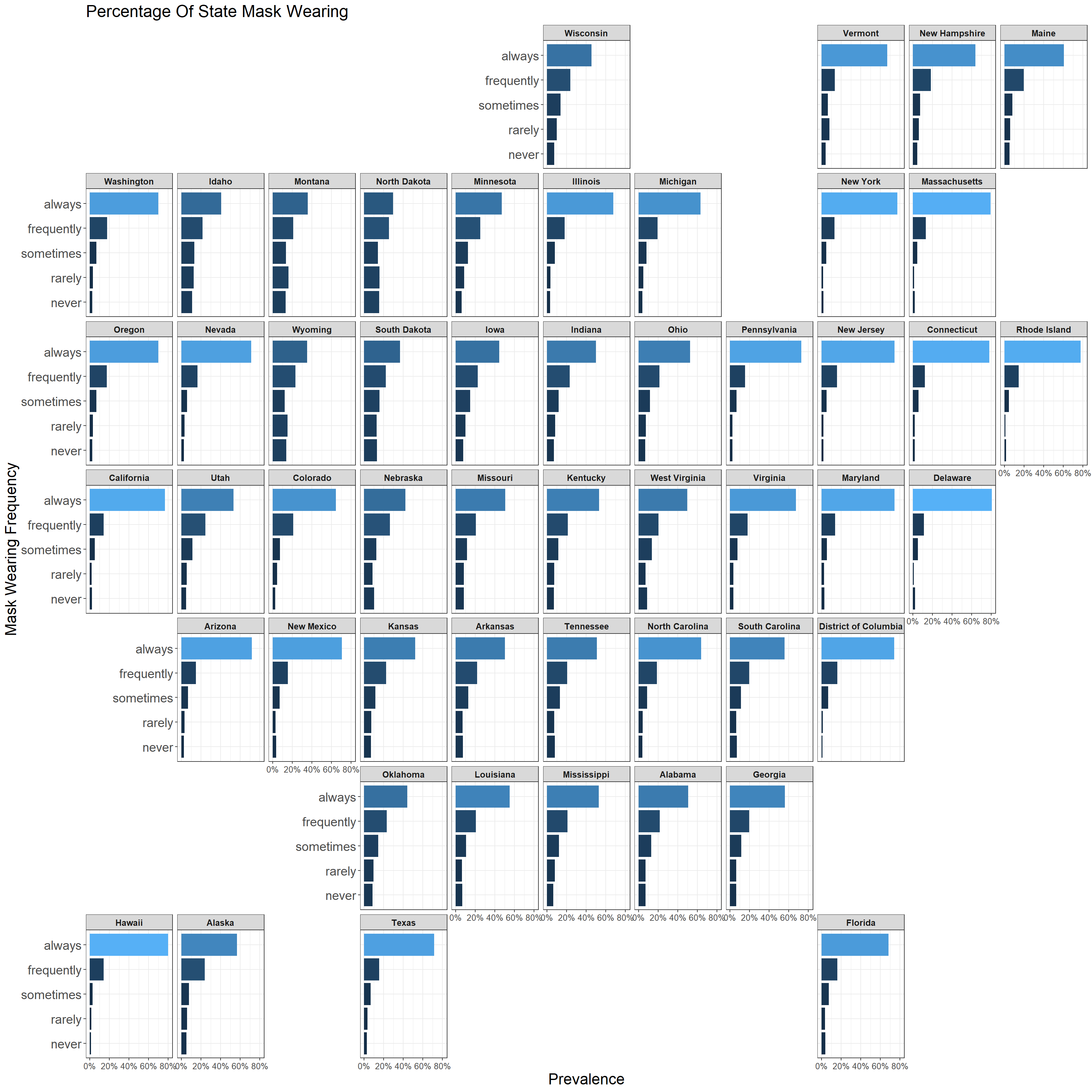
Based on the plot above, it is easy to visualize that states located on both coasts have a relative higher always and frequently mask-wearing percents. Their counterparts in the middle are lower in this regard.
Conclusion
This is an interesting real-world project that combines few datasets to make the final visual product, which conveys information about the mask-wearing situation in each state. We started from the county level and upgraded the relevant statistics to the state level, and finally the public opinion on mask-wearing is shown through a collection of geo-facet bar charts. A number of joins and some reshaping method (pivot_longer()), which are the basic data science skills, have been used in the project and hopefully, some techniques presented here can shed some light on data wrangling and visualization.