Horror Movies Data Visualization with Text Mining and LASSO Model
In this blog post, we will analyze a horror movie dataset from TidyTuesday by visualizing some interesting metrics and by using text mining and applying LASSO model on predicting movie ratings.
Data Introduction and Processing
First, load the necessary libraries we need for the analysis.
library(tidyverse)
library(lubridate)
library(tidytext)
library(broom)
library(glmnet)
library(Matrix)
library(scales)
Then, the dataset is loaded and we can see the first few rows.
movies <- read_csv("https://raw.githubusercontent.com/rfordatascience/tidytuesday/master/data/2019/2019-10-22/horror_movies.csv")

head(movies)
## # A tibble: 6 x 12
## title genres release_date release_country movie_rating review_rating
## <chr> <chr> <chr> <chr> <chr> <dbl>
## 1 Gut (2012) Drama| H~ 26-Oct-12 USA NA 3.9
## 2 The Hauntin~ Horror 13-Jan-17 USA NA NA
## 3 Sleepwalkin~ Horror 21-Oct-17 Canada NA NA
## 4 Treasure Ch~ Comedy| ~ 23-Apr-13 USA NOT RATED 3.7
## 5 Infidus (20~ Crime| D~ 10-Apr-15 USA NA 5.8
## 6 In Extremis~ Horror| ~ 2017 UK NA NA
## # ... with 6 more variables: movie_run_time <chr>, plot <chr>, cast <chr>,
## # language <chr>, filming_locations <chr>, budget <chr>Then use skim() from skimr package to give an overview of the dataset.
skimr::skim(movies)| Name | movies |
| Number of rows | 3328 |
| Number of columns | 12 |
| _______________________ | |
| Column type frequency: | |
| character | 11 |
| numeric | 1 |
| ________________________ | |
| Group variables | None |
Variable type: character
| skim_variable | n_missing | complete_rate | min | max | empty | n_unique | whitespace |
|---|---|---|---|---|---|---|---|
| title | 0 | 1.00 | 8 | 62 | 0 | 3303 | 0 |
| genres | 1 | 1.00 | 6 | 79 | 0 | 261 | 0 |
| release_date | 0 | 1.00 | 4 | 9 | 0 | 1332 | 0 |
| release_country | 0 | 1.00 | 2 | 20 | 0 | 72 | 0 |
| movie_rating | 1877 | 0.44 | 1 | 9 | 0 | 11 | 0 |
| movie_run_time | 544 | 0.84 | 6 | 7 | 0 | 113 | 0 |
| plot | 1 | 1.00 | 20 | 547 | 0 | 3310 | 0 |
| cast | 14 | 1.00 | 11 | 308 | 0 | 3296 | 0 |
| language | 71 | 0.98 | 4 | 64 | 0 | 187 | 0 |
| filming_locations | 1232 | 0.63 | 2 | 125 | 0 | 1171 | 0 |
| budget | 2094 | 0.37 | 2 | 18 | 0 | 417 | 0 |
Variable type: numeric
| skim_variable | n_missing | complete_rate | mean | sd | p0 | p25 | p50 | p75 | p100 | hist |
|---|---|---|---|---|---|---|---|---|---|---|
| review_rating | 252 | 0.92 | 5.08 | 1.47 | 1 | 4 | 5 | 6.1 | 9.8 | ▁▆▇▃▁ |
Keep in mind that there are some missing values in the dataset, and this means na.rm = TRUE is needed when summary results related to the missing-value column go awry.
Another thing we have noticed is that release_date column is a char rather than date column. Also, its formats are not consistent in a way that some entries are date with year, month and day, but others only include year. To deal with this, using parse_date_time is an ideal option.
movies$release_date <- parse_date_time(movies$release_date,
         orders=guess_formats(movies$release_date, c('dmy', 'y')))
budget is not a numeric column rather than a char string.
movies$budget <- parse_number(movies$budget)Data Visualization
movies %>%
  mutate(year = year(release_date)) %>%
  count(release_country, year, sort = TRUE) %>%
  mutate(release_country = fct_lump(release_country, n = 15, w = n),
         release_country = fct_reorder(release_country, n)) %>%
  ggplot(aes(n, release_country, fill = release_country)) +
  geom_col() +
  facet_wrap(~year) +
  theme_bw() +
  theme(
    strip.text = element_text(face = "bold"),
    legend.position = "none"
  ) +
  labs(x = "# of horror movies", y = NULL, title = "Yearly # of Horror Movies Produced by Each Country")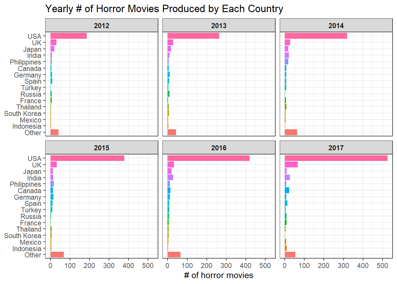
movies %>%
  mutate(year = year(release_date)) %>%
  count(language, year, sort = TRUE) %>%
  mutate(language = fct_lump(language, n = 15, w = n),
         language = fct_reorder(language, n)) %>%
  ggplot(aes(n, language, fill = language)) +
  geom_col() +
  facet_wrap(~year) +
  theme_bw() +
  theme(
    strip.text = element_text(face = "bold"),
    legend.position = "none"
  ) +
  labs(x = "# of horror movies", y = NULL, title = "Yearly # of Horror Movies Produced in Each Language")
It looks like from 2012 to 2017, USA produced the most number of horror movies in each year compared to other countries, and English horror movies were the most in all these years. This is consistent, as movies produced by USA are primarily English.
movies %>%
  mutate(release_country = fct_lump(release_country, 15)) %>%
  ggplot(aes(release_country, budget)) +
  geom_boxplot() +
  coord_flip() +
  theme_bw() +
  theme(
    axis.title.y = element_blank()
  ) +
  scale_y_continuous(labels = dollar)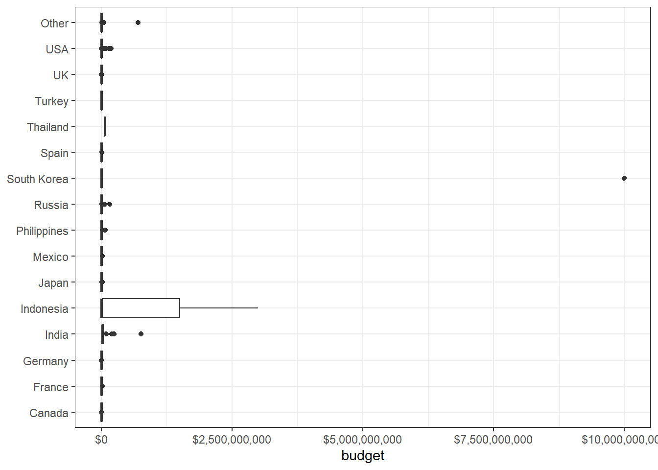
The above box plot is not informative in a way that a salient outlier overshadows all other data points. In such a case, using a log transformation can give us more information about movie budgets related to each country.
movies %>%
  mutate(release_country = fct_lump(release_country, 20),
         release_country = fct_reorder(release_country, log10(budget), median, na.rm = TRUE)) %>%
  ggplot(aes(release_country, log10(budget), fill = release_country)) +
  geom_boxplot() +
  coord_flip() +
  theme_bw() +
  theme(
    legend.position = "none"
  ) +
  labs(y = "budget (log10-scale)", x = NULL, title = "20 Country-wise Movie Budget")+
  scale_y_continuous(labels = dollar)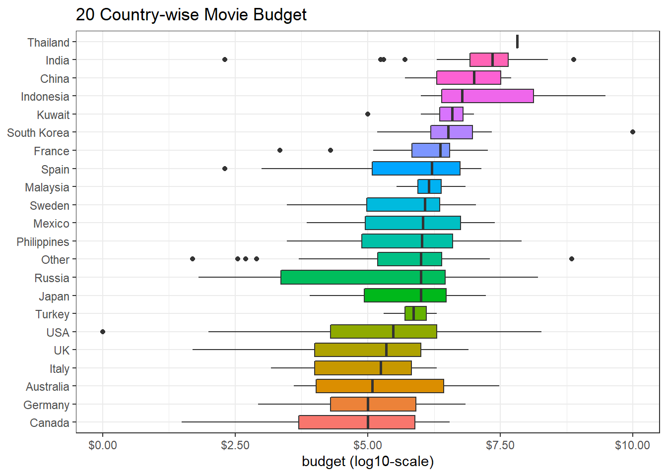
movies %>%
  ggplot(aes(budget, review_rating)) +
  geom_point() +
  scale_x_log10(labels = dollar) +
  geom_smooth(method = "lm") +
  theme_bw() +
  labs(x = "budget (log10 scale)")
Interestingly enough, there is no relationship between budget and review_rating. This is counter-intuitive, as investing more budget on a movie should generally have better ratings. However, this is not the case based on the plot shown above.
Text Analysis and Lasso Model
With a few minor changes, all the code below is largely referenced from David Robinson’s Github page for learning purposes.
movies_processed <- movies %>%
  separate(plot, c("director", "cast_sentence", "plot"), extra = "merge", sep = "\\. ", fill = "right") %>%
  filter(!is.na(review_rating)) %>%
  mutate(director = str_remove(director, "Directed by "))
movies_unnested <- movies_processed %>%
unnest_tokens(word, plot) %>%
anti_join(stop_words, by = "word")
movies_unnested %>%
group_by(word) %>%
summarize(movies = n(),
avg_rating = mean(review_rating, na.rm = TRUE)) %>%
arrange(desc(movies)) %>%
filter(movies > 100) %>%
mutate(word = fct_reorder(word, avg_rating)) %>%
ggplot(aes(avg_rating, word)) +
geom_point() +
theme_bw() +
labs(x = "average rating", y = "description word", title = "Description Words and Movie Ratings",
subtitle = "Word apeared in movie description and average rating of all movies whose description includes the word")## `summarise()` ungrouping output (override with `.groups` argument)
This is my first time using cast_sparse for making a document-term matrix (or DTM). For more information about DTM, please visit Text Mining with R or Wikipedia
movie_word_matrix <- movies_unnested %>%
  filter(!is.na(review_rating)) %>%
  add_count(word) %>%
  filter(n >= 20) %>%
  count(title, word) %>%
  cast_sparse(title, word, n)

rating <- movies$review_rating[match(rownames(movie_word_matrix), movies$title)]

lasso_model <- cv.glmnet(movie_word_matrix, rating)

plot(lasso_model)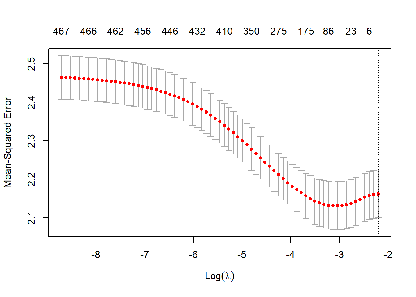
tidy(lasso_model$glmnet.fit) %>%
  filter(lambda == lasso_model$lambda.min,
         term != "(Intercept)") %>%
  mutate(term = fct_reorder(term, estimate)) %>%
  ggplot(aes(term, estimate)) +
  geom_col() +
  coord_flip() +
  ggtitle("Words Contributing to Movie Ratings")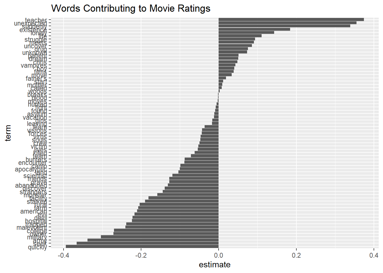
Now, we can select a few words from the above plot to visualize their relations between estimates and lambda values.
tidy(lasso_model$glmnet.fit) %>%
  filter(term %in% c("quickly", "seek", "army", "teacher", "unexpected", "friends", "evil")) %>%
  ggplot(aes(lambda, estimate, color = term)) +
  geom_line() +
  geom_vline(xintercept = lasso_model$lambda.min) +
  geom_hline(yintercept = 0, lty = 2)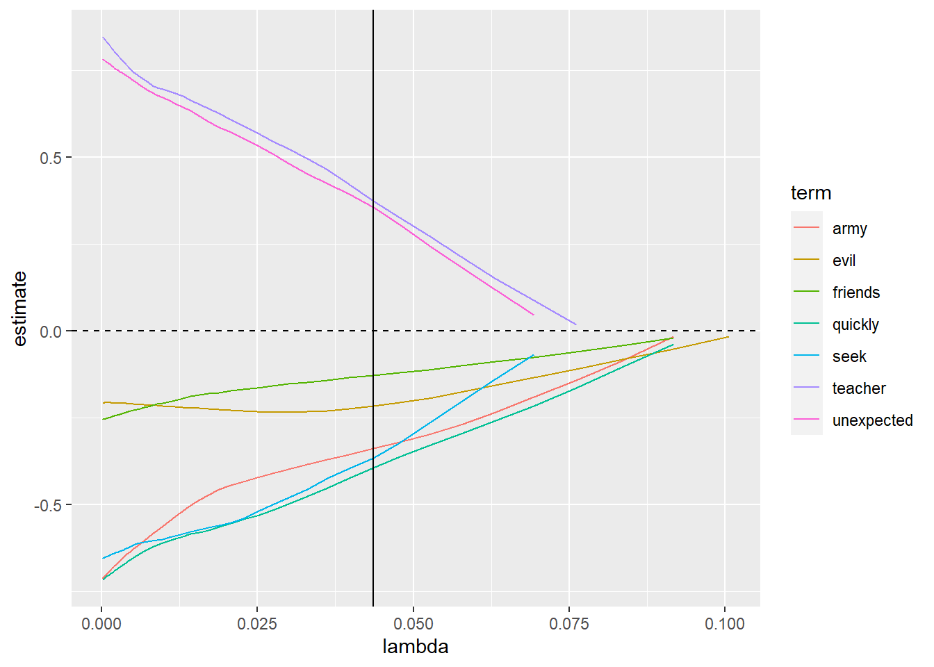
Now we throw all features into a LASSO model and see how each feature contributes to movie rating.
# The following code David Robinson used gather() function, but pivot_longer() should be more contemporary, #though achieving the same goal.
features <- movies_processed %>%
  filter(!is.na(review_rating)) %>%
  select(title, genres, director, cast, movie_rating, language, release_country) %>%
  mutate(director = str_remove(director, "Directed by ")) %>%
  pivot_longer(!title, names_to = "type", values_to = "value") %>%
  #gather(type, value, -title) %>% View()
  filter(!is.na(value)) %>%
  separate_rows(value, sep = "\\| ?") %>%
  unite(feature, type, value, sep = ": ") %>%
  mutate(n = 1)

movie_feature_matrix <- movies_unnested %>%
  filter(!is.na(review_rating)) %>%
  count(title, feature = paste0("word: ", word)) %>%
  bind_rows(features) %>%
  add_count(feature) %>%
  filter(nn >= 10) %>%
  cast_sparse(title, feature)
## Storing counts in `nn`, as `n` already present in input
## i Use `name = "new_name"` to pick a new name.rating <- movies$review_rating[match(rownames(movie_feature_matrix), movies$title)]
feature_lasso_model <- cv.glmnet(movie_feature_matrix, rating)
plot(feature_lasso_model)
tidy(feature_lasso_model$glmnet.fit) %>%
  filter(lambda == feature_lasso_model$lambda.1se,
         term != "(Intercept)") %>%
  mutate(term = fct_reorder(term, estimate)) %>%
  ggplot(aes(term, estimate)) +
  geom_col() +
  coord_flip() +
  labs(x = "",
       y = "Coefficient for predicting movie rating",
       title = "What affects a horror movie rating?",
       subtitle = "Based on a lasso regression to predict IMDb ratings of ~3000 movies")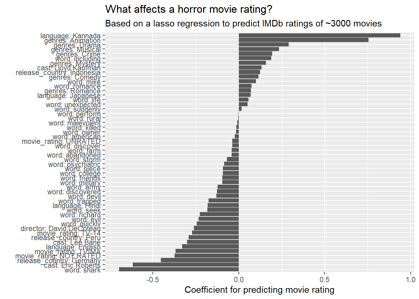
language:Kannada contributes the most to movie ratings in a positive way and word:shark in a negative way.
Conclusion
In this blog post, we analyzed the horror movie dataset from TidyTuesday through visualization and LASSO model predicting movie rating based on a number of features. The notion of document-term matrix is a tad difficult to use, especially combining it with cv.glmnet(). The LASSO model is a highly useful and practical prediction model that gives us great flexibility, and through this post, it can shed some light on how to use the model and we can follow the similar steps in the future when encountering analogous prediction problems.