Movie Profits Analysis
The dataset we will analyze is from TidyTuesday about movie profits for a slew of movie distributors with various genres.
Data Introduction
Let’s load the libraries and set the theme as theme_bw().
library(tidyverse)
library(lubridate)
library(scales)
library(tidytext)
theme_set(theme_bw())
Load the dataset below and some regular data processing steps are needed after exploring it.
movie_profit_raw  <- read_csv("https://raw.githubusercontent.com/rfordatascience/tidytuesday/master/data/2018/2018-10-23/movie_profit.csv") %>%
  select(-X1) %>%
  mutate(domestic_profit = domestic_gross - production_budget,
         world_profit = worldwide_gross - production_budget)

head(movie_profit_raw)
## # A tibble: 6 x 10
## release_date movie production_budg~ domestic_gross worldwide_gross distributor
## <chr> <chr> <dbl> <dbl> <dbl> <chr>
## 1 6/22/2007 Evan~ 175000000 100289690 174131329 Universal
## 2 7/28/1995 Wate~ 175000000 88246220 264246220 Universal
## 3 5/12/2017 King~ 175000000 39175066 139950708 Warner Bro~
## 4 12/25/2013 47 R~ 175000000 38362475 151716815 Universal
## 5 6/22/2018 Jura~ 170000000 416769345 1304866322 Universal
## 6 8/1/2014 Guar~ 170000000 333172112 771051335 Walt Disney
## # ... with 4 more variables: mpaa_rating <chr>, genre <chr>,
## # domestic_profit <dbl>, world_profit <dbl>skimr::skim(movie_profit_raw)| Name | movie_profit_raw |
| Number of rows | 3401 |
| Number of columns | 10 |
| _______________________ | |
| Column type frequency: | |
| character | 5 |
| numeric | 5 |
| ________________________ | |
| Group variables | None |
Variable type: character
| skim_variable | n_missing | complete_rate | min | max | empty | n_unique | whitespace |
|---|---|---|---|---|---|---|---|
| release_date | 0 | 1.00 | 8 | 10 | 0 | 1768 | 0 |
| movie | 0 | 1.00 | 1 | 35 | 0 | 3400 | 0 |
| distributor | 48 | 0.99 | 3 | 22 | 0 | 201 | 0 |
| mpaa_rating | 137 | 0.96 | 1 | 5 | 0 | 4 | 0 |
| genre | 0 | 1.00 | 5 | 9 | 0 | 5 | 0 |
Variable type: numeric
| skim_variable | n_missing | complete_rate | mean | sd | p0 | p25 | p50 | p75 | p100 | hist |
|---|---|---|---|---|---|---|---|---|---|---|
| production_budget | 0 | 1 | 33284743 | 34892391 | 2.5e+05 | 9000000 | 20000000 | 45000000 | 175000000 | ▇▂▁▁▁ |
| domestic_gross | 0 | 1 | 45421793 | 58825661 | 0.0e+00 | 6118683 | 25533818 | 60323786 | 474544677 | ▇▁▁▁▁ |
| worldwide_gross | 0 | 1 | 94115117 | 140918242 | 0.0e+00 | 10618813 | 40159017 | 117615211 | 1304866322 | ▇▁▁▁▁ |
| domestic_profit | 0 | 1 | 12137050 | 48201237 | -1.6e+08 | -9982528 | 530470 | 23237389 | 449998007 | ▁▇▁▁▁ |
| world_profit | 0 | 1 | 60830374 | 120934891 | -1.6e+08 | -2279629 | 16008693 | 74830111 | 1134866322 | ▇▂▁▁▁ |
With the data column, it is always nice to transfrom it into date column by using the nifty mdy() from lubridate package.
movie_profit_raw$release_date <- mdy(movie_profit_raw$release_date)Data Visualization
movie_profit_raw %>%
  ggplot(aes(domestic_gross)) +
  geom_histogram()
movie_profit_raw %>%
  ggplot(aes(worldwide_gross)) +
  geom_histogram()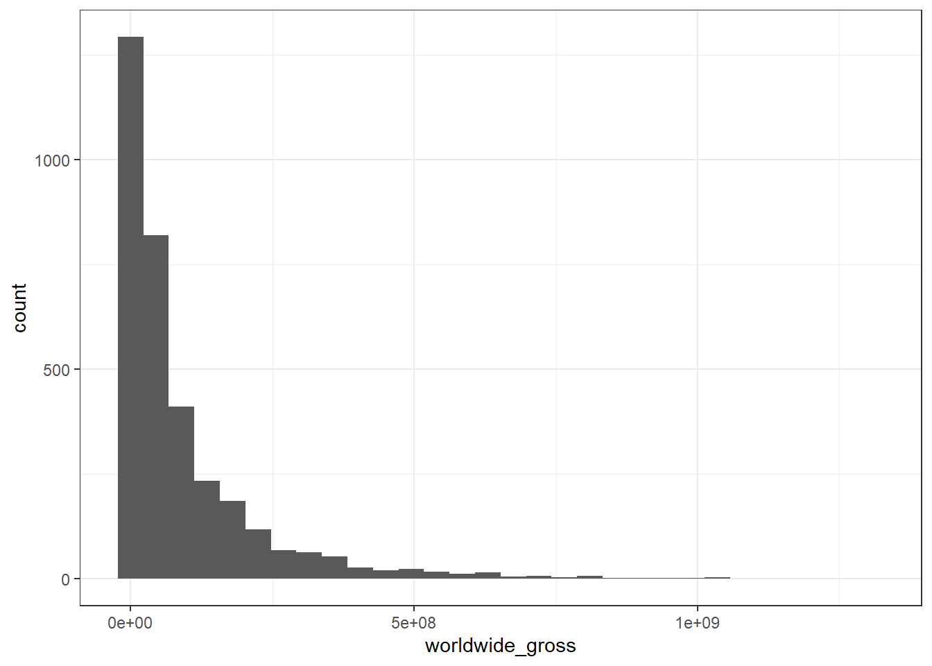
Based on the histograms above, it is always expected that income or revenue is always needed to have log-transformation.
gross_box <- function(gross, x = "", title = ""){
  gross <- enquo(gross)
  movie_profit_raw %>%
  filter(!is.na(distributor)) %>%
  mutate(distributor = fct_lump(distributor, n = 20)) %>%
  ggplot(aes(log10(!!gross), reorder_within(distributor, log10(!!gross), genre, fun = median),
             fill = distributor)) +
  geom_boxplot() +
  facet_wrap(~genre, scales = "free_y") +
  scale_x_continuous(labels =  dollar) +
  theme(
    legend.position = "none",
    strip.text = element_text(size = 15, face = "bold")
  ) +
  scale_y_reordered() +
  labs(x = paste(x, "(log10 scale)"), y = NULL, title = title)

}

gross_box(domestic_gross, x = "domestic gross", title = "20 Distributors Domestic Gross Faceted by Genre")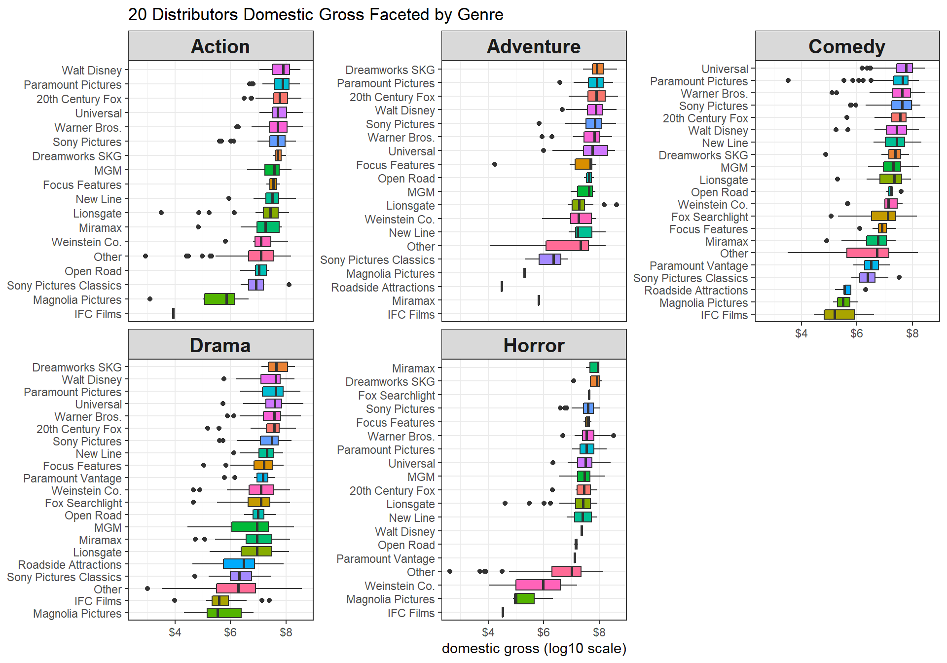
gross_box(worldwide_gross, x = "worldwide gross", title = "20 Distributors Worldwide Gross Faceted by Genre")
movie_gross <- function(gross, x = "", title = ""){
  gross <- enquo(gross)
  movie_profit_raw %>%
  mutate(year = year(release_date)) %>%
  filter(year > 2010, !!gross > 0) %>%
  group_by(year, genre, distributor) %>%
  summarize(median = median(!!gross, na.rm = TRUE),
            min = min(!!gross, na.rm = TRUE),
            max = max(!!gross, na.rm = TRUE)) %>%
  ungroup() %>%
  mutate(distributor = fct_lump(distributor, n = 5)) %>%
  filter(distributor != "Other") %>%
  #pivot_longer(cols = c(median, min, max), names_to = "metric", values_to = "domestic_gross") %>%
  ggplot(aes(median, distributor, color = distributor)) +
  geom_point(aes(size = median)) +
  geom_errorbar(aes(xmin = min, xmax = max)) +
  facet_grid(year ~ genre) +
  theme(
    strip.text = element_text(size = 12, face = "bold"),
    axis.text.x = element_text(angle = 10)
  ) +
  scale_x_continuous(labels = dollar, n.breaks = 3) +
  labs(color = NULL, x = x, y = NULL, title = title,
       subtitle = "Error Bars represent the smallest and largest values") +
  scale_size_continuous(labels = dollar)

}

movie_gross(domestic_gross, x = "domestic gross", title = "Domestic Gross Faceted by Genre and Year")
movie_gross(worldwide_gross, x = "world gross", title = "Worldwide Gross Faceted by Genre and Year")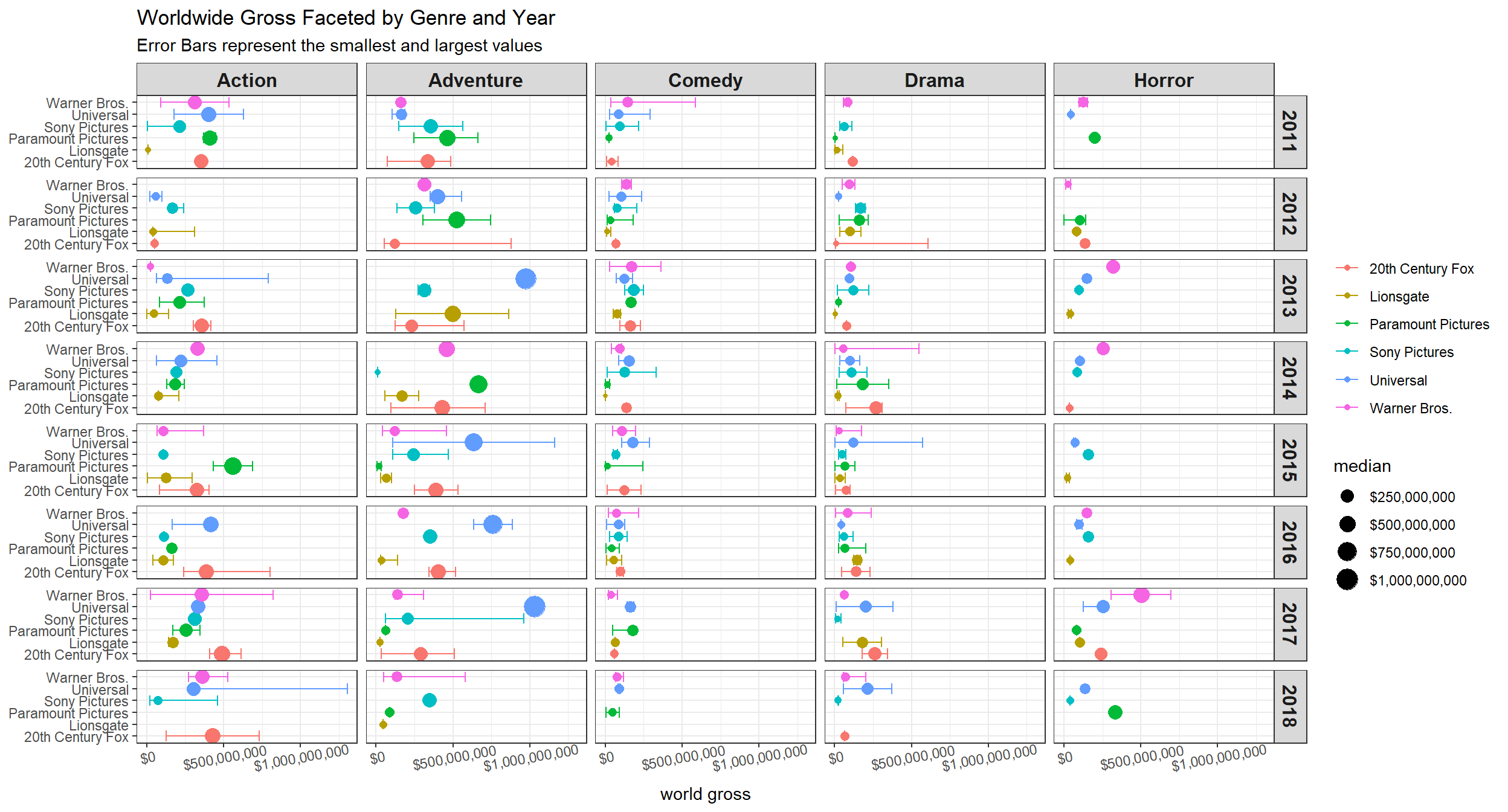
The above box plots and errorbar plots are self-explanatory.
budget_profit <- function(profit, title = ""){
  profit <- enquo(profit)
  movie_profit_raw  %>%
  arrange(desc(domestic_profit, world_profit)) %>%
  ggplot(aes(production_budget, !!profit)) +
  geom_point() +
  geom_smooth(method = "lm") +
  geom_text(aes(label = movie, color = distributor), check_overlap = TRUE) +
  theme(
    legend.position = "none"
  ) +
  labs(x = "production budget", y = "profits", title = title)+
  scale_x_continuous(labels = dollar) +
  scale_y_continuous(labels = dollar)

}

budget_profit(domestic_profit, title = "Domestic Profits") 
budget_profit(world_profit, title = "Worldwide Profits")
What is interesting from the scatter plots about the domestic and worldwide profits is that there is no relationship at all between production budget and domestic profits; and there is a slight upward trend between budget and worldwide profits.
Ratings
ratings <- function(y_axis, y, title = title){
  y_axis <- enquo(y_axis)
  movie_profit_raw %>%
  ggplot(aes(mpaa_rating, !!y_axis, fill = mpaa_rating)) +
  geom_boxplot() +
  theme(
    legend.position = "none"
  ) +
  labs(x = "mpaa rating", y = y, title = title) +
  scale_y_continuous(labels = dollar)
}

ratings(production_budget, y = "production budget", title = "Production Budget with MPAA Rating")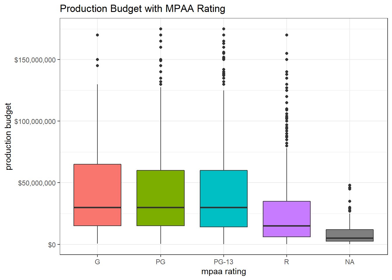
ratings(domestic_profit, y = "Domestic Profits", title = "Domestic Profits with MPAA Rating")
ratings(world_profit, y = "Worldwide Profits", title = "World Profits with MPAA Rating")
Transforming Year to Decade
There is a trick that transform year to decade in R, and that is 10*floor(year/10). Now instead of working on year, decade can give us a more general view on this dataset.
movie_profit_raw %>%
  mutate(year = year(release_date),
          decade = 10 * floor(year/ 10),
          distributor = fct_lump(distributor, 5)) %>%
  filter(!is.na(distributor), decade >= 1960, distributor != "Other") %>%
  count(distributor, decade, genre, sort = TRUE) %>%
  ggplot(aes(decade, n, fill = distributor)) +
  geom_col() +
  facet_grid(distributor~genre) +
  theme_bw() +
  theme(
    legend.position = "none",
    strip.text = element_text(size = 10, face = "bold")
  ) +
  labs(y = "# of movies") +
  scale_x_continuous(breaks = seq(1960, 2010, by = 10))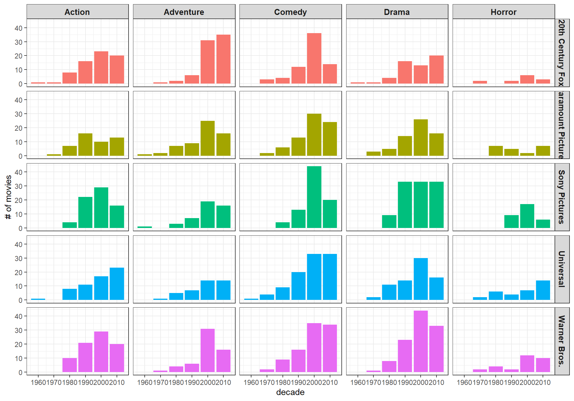
Others
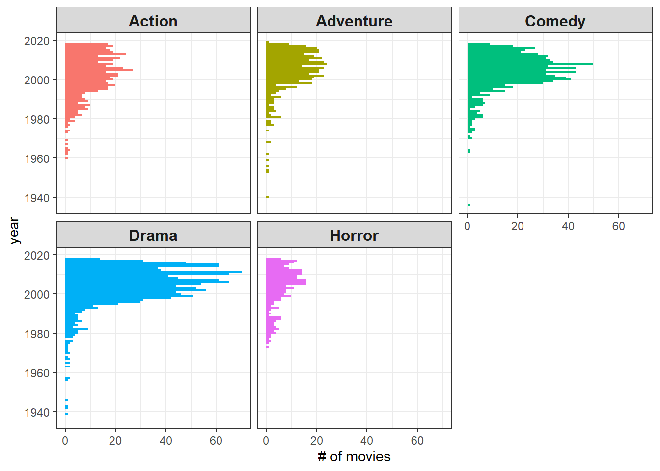
What are the most common genres over time?
movie_profit_raw %>%
  mutate(year = year(release_date)) %>%
  count(genre, year, sort = TRUE) %>%
  ggplot(aes(year, n, fill = genre)) +
  geom_col() +
  coord_flip() +
  facet_wrap(~genre) +
  labs(y = "# of movies") +
  theme(
    strip.text = element_text(size = 12, face = "bold"),
    legend.position = "none"
  ) +
  scale_x_continuous(n.breaks = 6)