R and R Package Download Analysis
R is a nice tool I use everyday for my data analysis work, especially those data science libraries such as tidyverse that have made my work productive. In this blog, we analyze R and R package downloads, and here is the dataset download link.
library(tidyverse)
library(lubridate)
library(scales)
library(countrycode)
theme_set(theme_bw())
r_raw <- read_csv("https://raw.githubusercontent.com/rfordatascience/tidytuesday/master/data/2018/2018-10-30/r_downloads_year.csv") %>%
select(-X1) %>%
mutate(country_name = countrycode(country, "iso2c", "country.name"))
head(r_raw)## # A tibble: 6 x 8
## date time size version os country ip_id country_name
## <date> <time> <dbl> <chr> <chr> <chr> <dbl> <chr>
## 1 2017-10-23 14:29:18 78171332 3.4.2 win ES 1 Spain
## 2 2017-10-23 14:29:22 20692638 3.4.2 win PT 2 Portugal
## 3 2017-10-23 14:29:57 972075 3.4.2 win PL 3 Poland
## 4 2017-10-23 14:30:00 1032203 3.0.3 win JP 4 Japan
## 5 2017-10-23 14:30:18 78171332 3.4.2 win CN 5 China
## 6 2017-10-23 14:30:50 64228612 3.4.2 osx US 6 United Statesskimr::skim(r_raw)| Name | r_raw |
| Number of rows | 938115 |
| Number of columns | 8 |
| _______________________ | |
| Column type frequency: | |
| character | 4 |
| Date | 1 |
| difftime | 1 |
| numeric | 2 |
| ________________________ | |
| Group variables | None |
Variable type: character
| skim_variable | n_missing | complete_rate | min | max | empty | n_unique | whitespace |
|---|---|---|---|---|---|---|---|
| version | 0 | 1.00 | 5 | 12 | 0 | 81 | 0 |
| os | 2598 | 1.00 | 3 | 3 | 0 | 3 | 0 |
| country | 22514 | 0.98 | 2 | 2 | 0 | 222 | 0 |
| country_name | 24672 | 0.97 | 4 | 42 | 0 | 218 | 0 |
Variable type: Date
| skim_variable | n_missing | complete_rate | min | max | median | n_unique |
|---|---|---|---|---|---|---|
| date | 0 | 1 | 2017-10-20 | 2018-10-20 | 2018-04-29 | 366 |
Variable type: difftime
| skim_variable | n_missing | complete_rate | min | max | median | n_unique |
|---|---|---|---|---|---|---|
| time | 0 | 1 | 0 secs | 86399 secs | 13:35:58 | 86387 |
Variable type: numeric
| skim_variable | n_missing | complete_rate | mean | sd | p0 | p25 | p50 | p75 | p100 | hist |
|---|---|---|---|---|---|---|---|---|---|---|
| size | 0 | 1 | 70506726.72 | 24997546.36 | 0 | 77266199 | 82375219 | 82968668 | 83702175 | ▁▁▁▁▇ |
| ip_id | 0 | 1 | 939.49 | 751.48 | 1 | 302 | 803 | 1434 | 3748 | ▇▅▃▁▁ |
Country-wise downloads
r_raw %>%
  mutate(year = year(date),
         ) %>%
  count(year, country_name, sort = TRUE) %>%
  filter(!is.na(country_name)) %>%
  mutate(
    country_name = fct_lump(country_name, n = 15, w = n),
    country_name = fct_reorder(country_name, n)
  ) %>%
  ggplot(aes(n, country_name, fill = country_name)) +
  geom_col(show.legend = FALSE)  +
  facet_wrap(~year) +
  theme(
    strip.text = element_text(size = 13)
  ) +
  scale_x_continuous(labels = comma) +
  labs(x = "# of R downloads", y = NULL, title = "Top 15 Countries R Downloads Faceted by Year")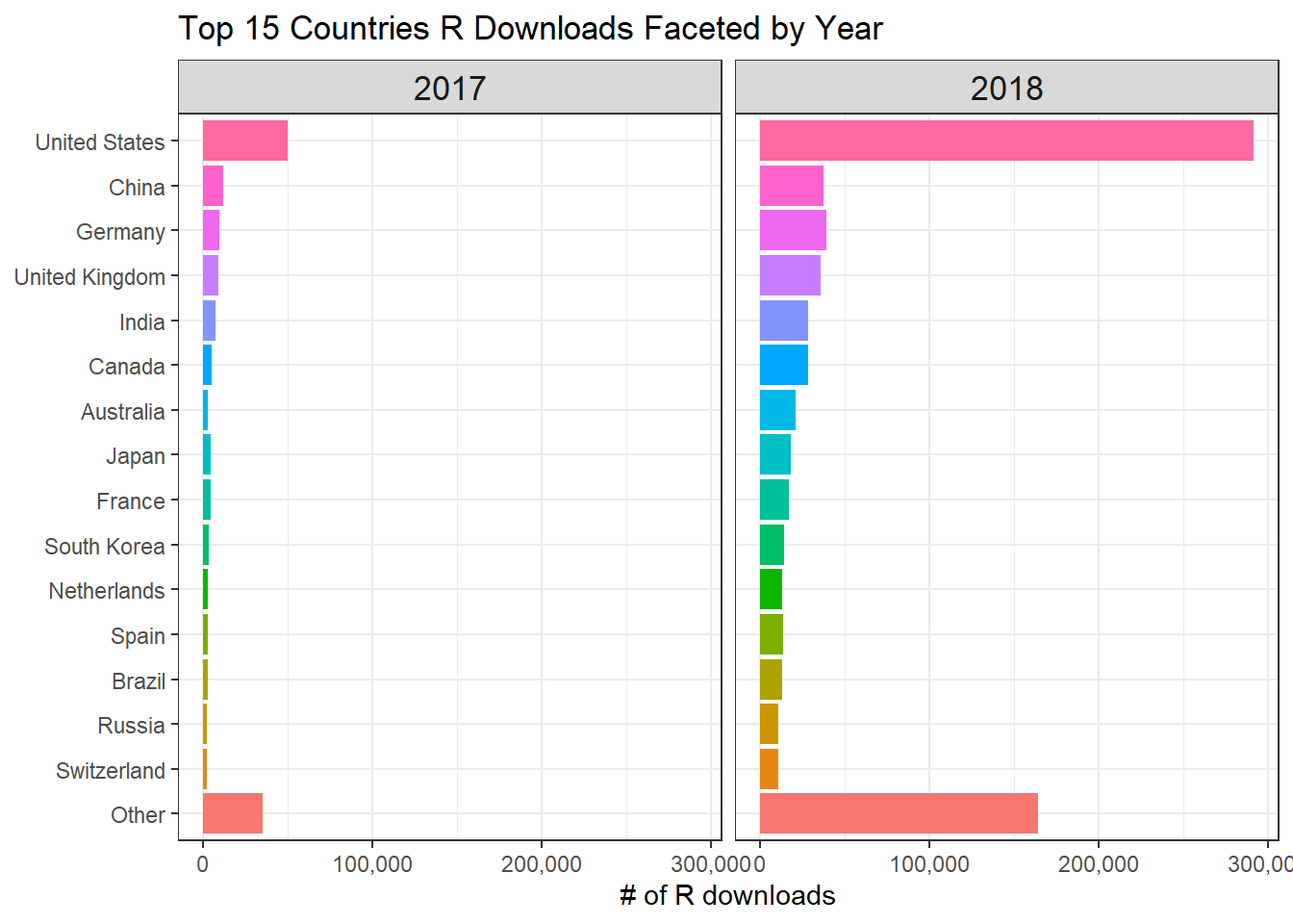
Operating Systems
r_raw %>%
  count(version, os, sort = T) %>%
  mutate(version = fct_lump(version, n = 15, w = n),
         version = fct_reorder(version, n)) %>%
  filter(!is.na(os)) %>%
  ggplot(aes(os, version, fill = n)) +
  geom_tile() +
  theme(
    axis.title = element_text(size = 15),
    axis.text = element_text(size = 12)
  ) +
labs(fill = "# of R downloads", title = "# of R Downloads with Different Versions and OS Platforms") 
r_raw %>%
  count(version, os, sort = T) %>%
  mutate(version = fct_lump(version, n = 15, w = n),
         version = fct_reorder(version, n)) %>%
  filter(!is.na(os)) %>%
  ggplot(aes(n, version, fill = version)) +
  geom_col(show.legend = FALSE) +
  facet_wrap(~os) +
  theme(
    strip.text = element_text(size = 13, face = "bold"),
    axis.title = element_text(size = 15),
    axis.text = element_text(size = 12)
  ) +
labs(x = "# of R downloads", title = "# of R Downloads with Different Versions and OS Platforms") 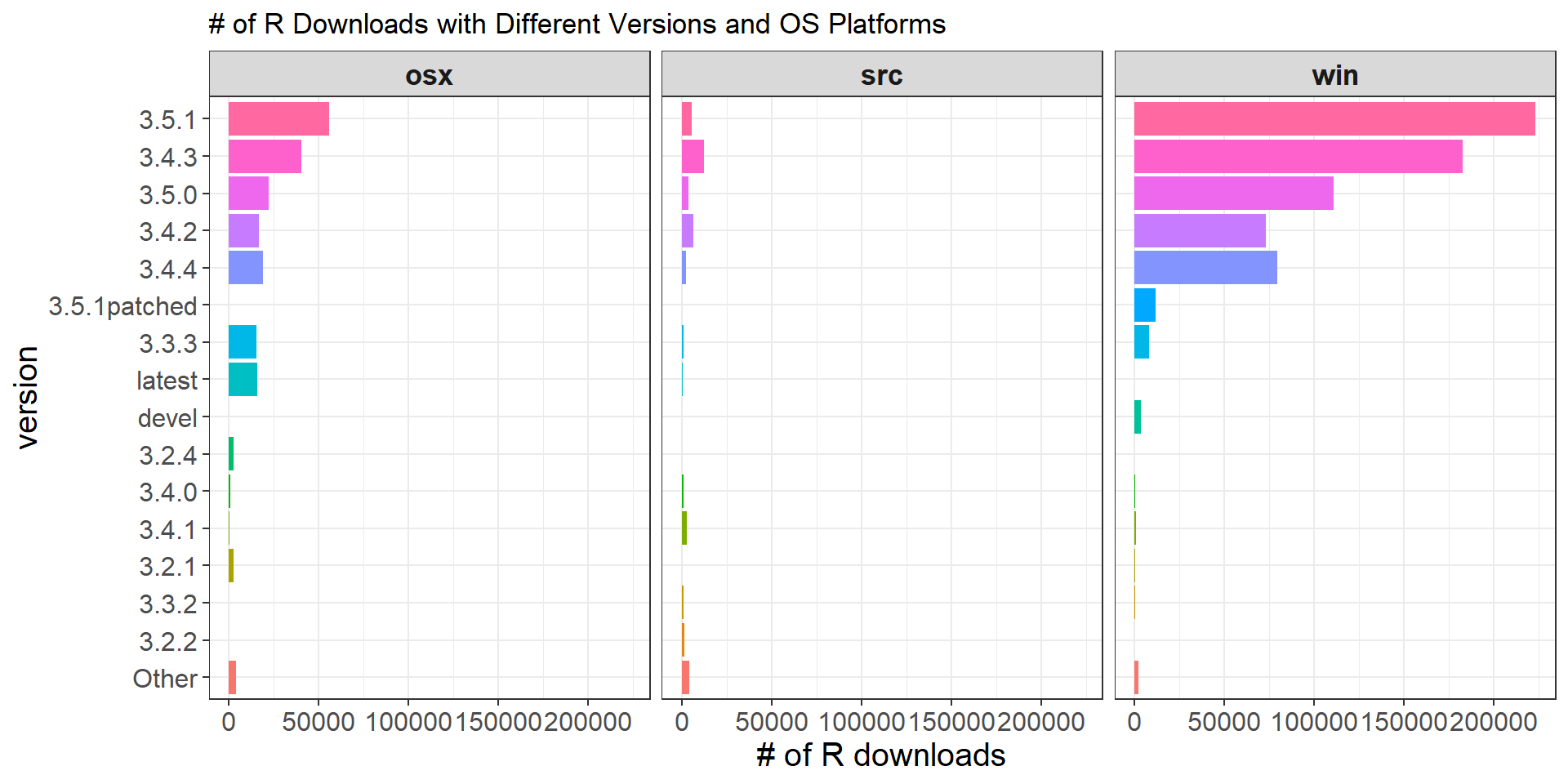
r_raw %>%
  group_by(os, date) %>%
  summarize(downloads = n()) %>%
  ggplot(aes(date, downloads, color = os)) +
  geom_line() +
  geom_point() +
  expand_limits(y = 0) +
  scale_x_date(date_breaks = "2 months") +
  geom_smooth(method = "lm") +
  ggtitle("Time-series Total # of R Downloads")
## `summarise()` regrouping output by 'os' (override with `.groups` argument)## `geom_smooth()` using formula 'y ~ x'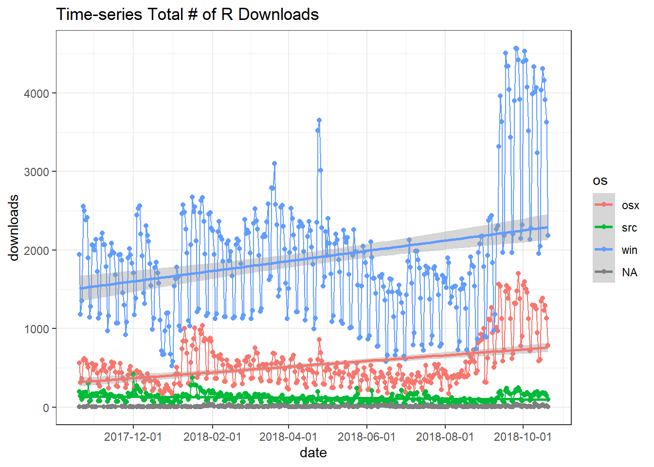
r_raw %>%
  group_by(os, date) %>%
  summarize(downloads = n()) %>%
  ggplot(aes(date, downloads, color = factor(year(date)))) +
  geom_line() +
  geom_point() +
  expand_limits(y = 0) +
  scale_x_date(date_breaks = "2 months") +
  geom_smooth(method = "lm") +
  labs(color = NULL) +
  ggtitle("Time-series Total # of R Downloads")
## `summarise()` regrouping output by 'os' (override with `.groups` argument)## `geom_smooth()` using formula 'y ~ x'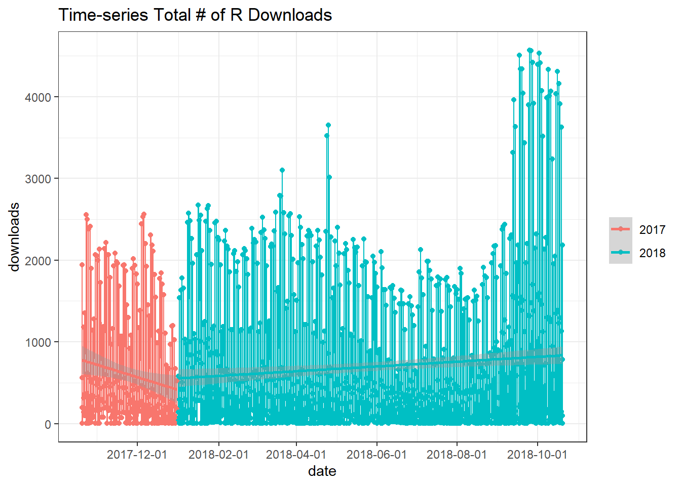
Package Size
r_raw %>%
  mutate(mb = size/10^6,
         version = fct_lump(version, 5)) %>%
  ggplot(aes(os, version, fill = mb)) +
  geom_tile() +
  theme(
    axis.title = element_text(size = 15),
    axis.text = element_text(size = 13)
  ) +
  labs(fill = "size (MB)")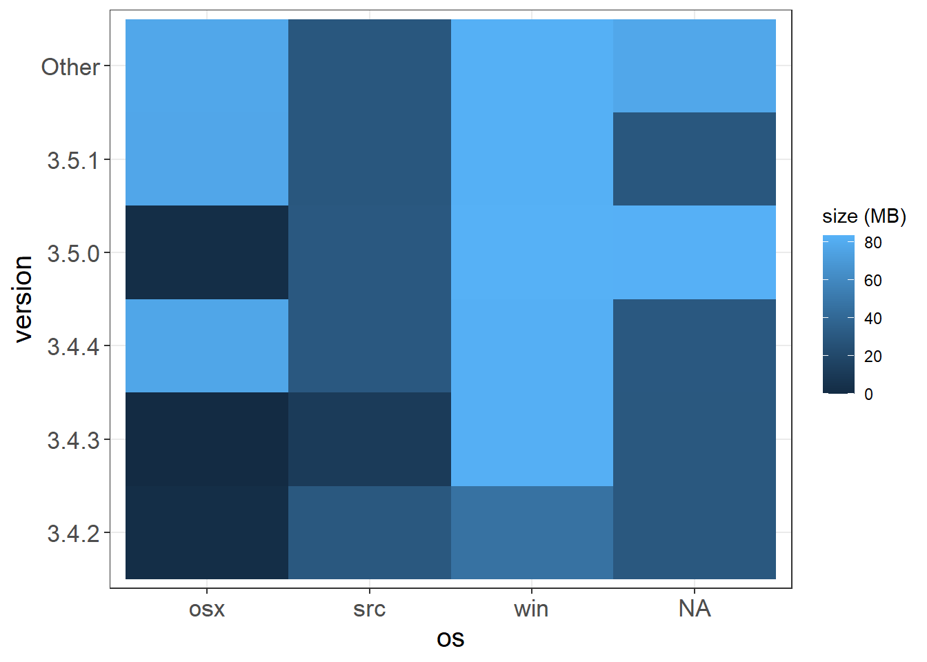
Weekday
r_raw %>%
  mutate(weekday = factor(weekdays(date), levels = c("Monday",
    "Tuesday", "Wednesday", "Thursday", "Friday", "Saturday", "Sunday")),
         hour = hour(time)) %>%
  group_by(weekday, hour) %>%
  summarize(downloads = n_distinct(ip_id)) %>%
  ggplot(aes(hour, downloads, color = weekday, linetype = weekday)) +
  geom_line(size = 1) +
  labs(color = NULL, linetype = NULL, y = "downloads (distinct IPs)")
## `summarise()` regrouping output by 'weekday' (override with `.groups` argument)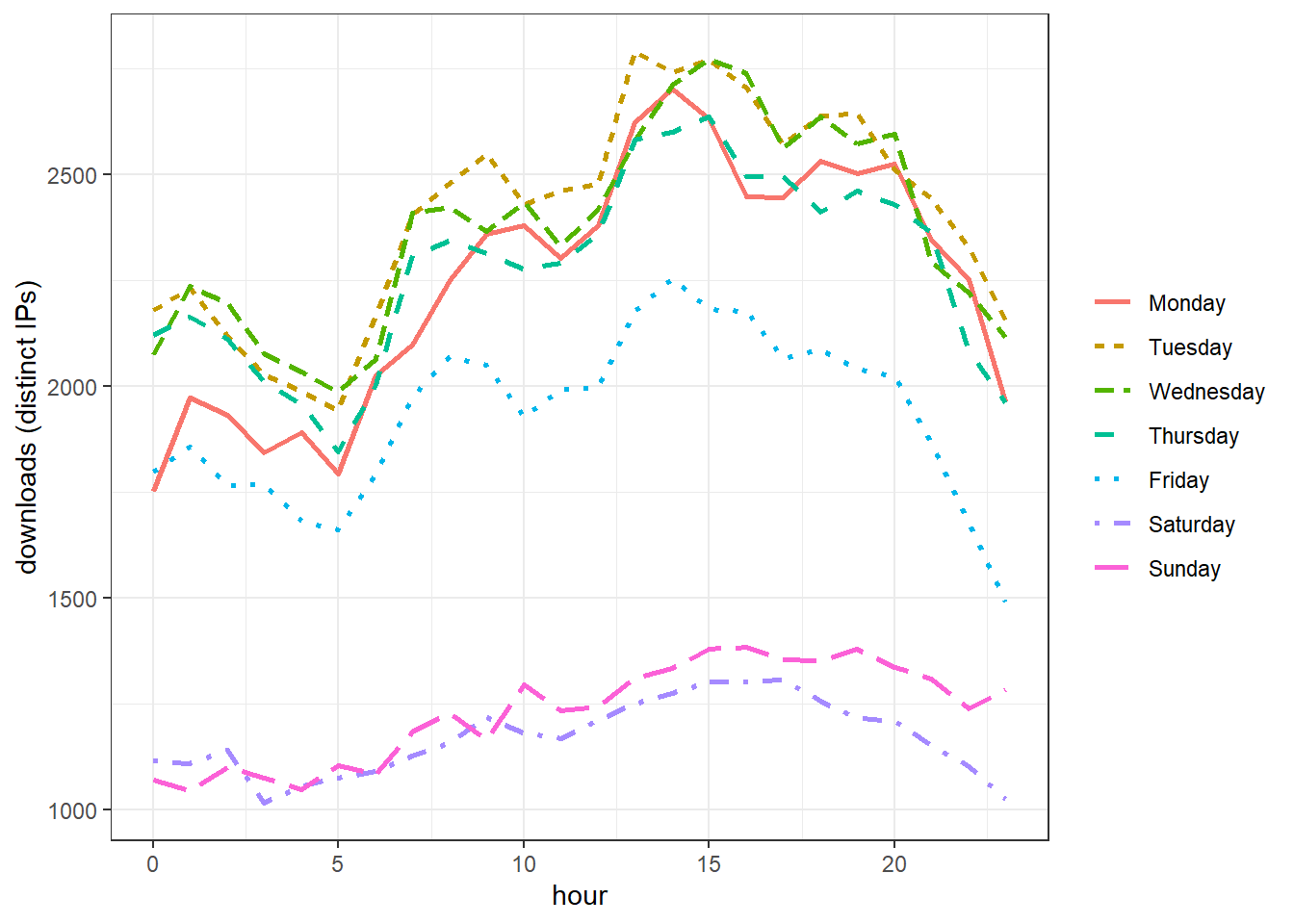
The following analysis is inspired by and adopted in part from David Robinson’s code, as when I was working on my analysis, I did not pay attention on ip_id column, which has some shocking number of duplicates.
r_raw %>%
  count(ip_id, sort = T)
## # A tibble: 3,748 x 2
## ip_id n
## <dbl> <int>
## 1 1 7093
## 2 7 5385
## 3 2 5158
## 4 5 4477
## 5 6 3756
## 6 10 3623
## 7 4 3341
## 8 12 2369
## 9 18 2295
## 10 3 2219
## # ... with 3,738 more rowsr_raw %>%
ggplot(aes(ip_id)) +
geom_histogram()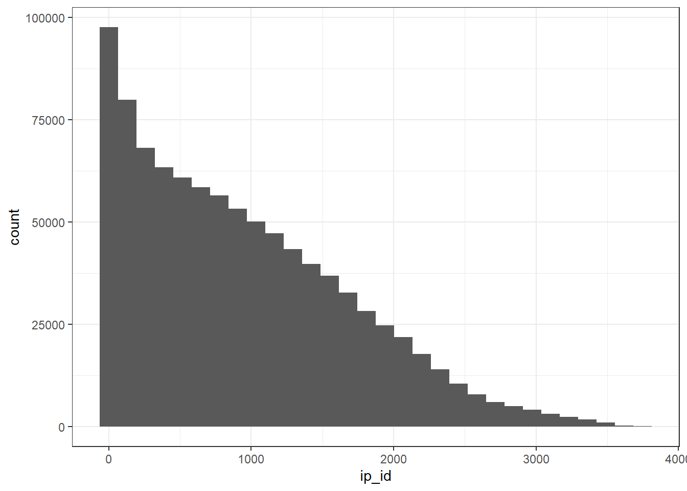
In his code, Robinson Used as.POSIXlt() to put date and time together assembling timestamp column datetime, but I found out that using ymd(date) + hms(time) can do the same job, and in some senese, is easier. Then using window function lag() trying to obtain the gaps within each ip_id.
r_raw %>%
  #mutate(datetime = as.POSIXlt(date) + time) %>%
  mutate(datetime = ymd(date) + hms(time)) %>%
  arrange(datetime) %>%
  group_by(ip_id) %>%
  mutate(gap = as.numeric(datetime - lag(datetime))) %>%
  filter(!is.na(gap)) %>%
  ggplot(aes(gap)) +
  geom_histogram() +
  geom_vline(color = "red", lty = 2, xintercept = 86400) +
  scale_x_log10(breaks = 60 ^ (0:4),
                labels = c("Second", "Minute", "Hour", "2.5 Days", "120 Days")) +
  scale_y_continuous(labels = comma)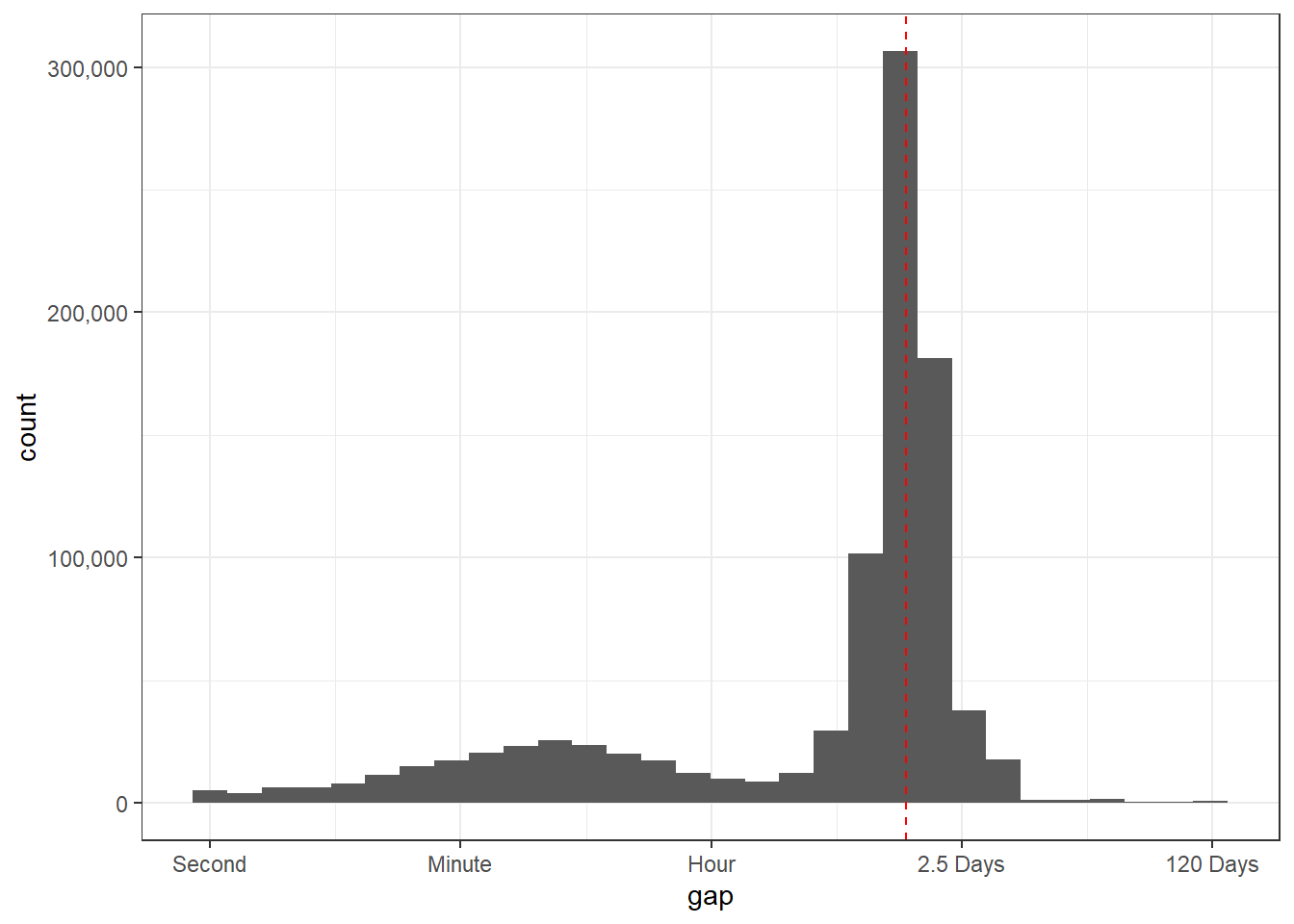
Note: First time using n_distinct() and floor_date().
r_raw %>%
  group_by(week = floor_date(date, "week", week_start = 1)) %>%
  summarize(n = n_distinct(ip_id)) %>%
  filter(week > min(week)) %>%
  ggplot(aes(week, n)) +
  geom_line() +
  expand_limits(y = 0) +
  labs(y = "# of R downloads per week (distinct IPs)")
Package Downloads
package_downloads <- read_csv("http://cran-logs.rstudio.com/2018/2018-10-27.csv.gz")

head(package_downloads)
## # A tibble: 6 x 10
## date time size r_version r_arch r_os package version country
## <date> <time> <dbl> <chr> <chr> <chr> <chr> <chr> <chr>
## 1 2018-10-27 22:43:31 2475672 3.5.1 x86_64 darwin1~ openssl 1.0.2 NA
## 2 2018-10-27 22:43:32 184625 3.5.1 x86_64 darwin1~ callr 3.0.0 NA
## 3 2018-10-27 22:43:31 266636 3.5.0 x86_64 linux-g~ fansi 0.4.0 US
## 4 2018-10-27 22:43:32 367563 3.5.0 x86_64 linux-g~ curl 3.2 US
## 5 2018-10-27 22:43:30 45922 3.4.1 x86_64 linux-g~ htmltoo~ 0.3.6 US
## 6 2018-10-27 22:43:30 57664 3.5.1 x86_64 darwin1~ viridis~ 0.3.0 NA
## # ... with 1 more variable: ip_id <dbl>package_downloads %>%
filter(country == "US") %>%
group_by(package) %>%
summarize(n = n_distinct(ip_id)) %>%
arrange(desc(n)) %>%
head(10) %>%
mutate(package = fct_reorder(package, n)) %>%
ggplot(aes(n, package, fill = package)) +
geom_col(show.legend = F) +
labs(x = "# of downloads")