US Wind Turbine Data Analysis
Tue, Sep 7, 2021
4-minute read
The dataset for this blog analysis is from TidyTuesday about wind turbine data across different states in the U.S. The dataset contains a number of technical terms that might not be easy to understand, but we can still use data science tools to analyze and visualize the data.
Data Introduction
library(tidyverse)
library(ggthemes)
library(geofacet)
theme_set(theme_bw())
wt <- read_csv("https://raw.githubusercontent.com/rfordatascience/tidytuesday/master/data/2018/2018-11-06/us_wind.csv",na = c("missing", "-9999", "n/a"))
head(wt)## # A tibble: 6 x 24
## case_id faa_ors faa_asn usgs_pr_id t_state t_county t_fips p_name p_year
## <dbl> <chr> <chr> <dbl> <chr> <chr> <chr> <chr> <dbl>
## 1 3073429 NA NA 4960 CA Kern County 06029 251 Wind 1987
## 2 3071522 NA NA 4997 CA Kern County 06029 251 Wind 1987
## 3 3073425 NA NA 4957 CA Kern County 06029 251 Wind 1987
## 4 3071569 NA NA 5023 CA Kern County 06029 251 Wind 1987
## 5 3005252 NA NA 5768 CA Kern County 06029 251 Wind 1987
## 6 3003862 NA NA 5836 CA Kern County 06029 251 Wind 1987
## # ... with 15 more variables: p_tnum <dbl>, p_cap <dbl>, t_manu <chr>,
## # t_model <chr>, t_cap <dbl>, t_hh <dbl>, t_rd <dbl>, t_rsa <dbl>,
## # t_ttlh <dbl>, t_conf_atr <dbl>, t_conf_loc <dbl>, t_img_date <chr>,
## # t_img_srce <chr>, xlong <dbl>, ylat <dbl>skimr::skim(wt)| Name | wt |
| Number of rows | 58185 |
| Number of columns | 24 |
| _______________________ | |
| Column type frequency: | |
| character | 10 |
| numeric | 14 |
| ________________________ | |
| Group variables | None |
Variable type: character
| skim_variable | n_missing | complete_rate | min | max | empty | n_unique | whitespace |
|---|---|---|---|---|---|---|---|
| faa_ors | 8405 | 0.86 | 9 | 9 | 0 | 49756 | 0 |
| faa_asn | 8095 | 0.86 | 13 | 17 | 0 | 49492 | 0 |
| t_state | 0 | 1.00 | 2 | 2 | 0 | 45 | 0 |
| t_county | 0 | 1.00 | 4 | 31 | 0 | 521 | 0 |
| t_fips | 0 | 1.00 | 5 | 5 | 0 | 631 | 0 |
| p_name | 0 | 1.00 | 3 | 42 | 0 | 1479 | 0 |
| t_manu | 3876 | 0.93 | 3 | 72 | 0 | 70 | 0 |
| t_model | 4469 | 0.92 | 2 | 14 | 0 | 260 | 0 |
| t_img_date | 24174 | 0.58 | 8 | 10 | 0 | 555 | 0 |
| t_img_srce | 0 | 1.00 | 4 | 16 | 0 | 4 | 0 |
Variable type: numeric
| skim_variable | n_missing | complete_rate | mean | sd | p0 | p25 | p50 | p75 | p100 | hist |
|---|---|---|---|---|---|---|---|---|---|---|
| case_id | 0 | 1.00 | 3040036.95 | 21727.20 | 3000001.00 | 3023351.00 | 3038762.00 | 3053909.00 | 3087216.00 | ▅▇▇▅▃ |
| usgs_pr_id | 15272 | 0.74 | 26396.60 | 13915.73 | 0.00 | 16301.00 | 27304.00 | 38130.00 | 49135.00 | ▆▆▇▇▇ |
| p_year | 62 | 1.00 | 2007.64 | 9.22 | 1981.00 | 2006.00 | 2010.00 | 2014.00 | 2018.00 | ▂▁▂▆▇ |
| p_tnum | 0 | 1.00 | 158.57 | 331.74 | 1.00 | 50.00 | 83.00 | 124.00 | 1831.00 | ▇▁▁▁▁ |
| p_cap | 3692 | 0.94 | 137.36 | 86.91 | 0.05 | 76.95 | 129.00 | 199.50 | 495.01 | ▇▇▅▁▁ |
| t_cap | 3694 | 0.94 | 1652.56 | 681.84 | 40.00 | 1500.00 | 1650.00 | 2000.00 | 6000.00 | ▂▇▁▁▁ |
| t_hh | 6625 | 0.89 | 77.31 | 12.87 | 18.20 | 80.00 | 80.00 | 80.00 | 130.00 | ▁▁▇▁▁ |
| t_rd | 4949 | 0.91 | 83.66 | 23.78 | 11.00 | 77.00 | 87.00 | 100.00 | 150.00 | ▁▂▇▆▁ |
| t_rsa | 4949 | 0.91 | 5941.47 | 2696.78 | 95.03 | 4656.63 | 5944.68 | 7853.98 | 17671.46 | ▃▇▆▁▁ |
| t_ttlh | 5062 | 0.91 | 120.70 | 22.83 | 9.10 | 118.60 | 123.40 | 131.40 | 200.30 | ▁▁▇▇▁ |
| t_conf_atr | 0 | 1.00 | 2.77 | 0.56 | 1.00 | 3.00 | 3.00 | 3.00 | 3.00 | ▁▁▁▁▇ |
| t_conf_loc | 0 | 1.00 | 2.95 | 0.31 | 1.00 | 3.00 | 3.00 | 3.00 | 3.00 | ▁▁▁▁▇ |
| xlong | 0 | 1.00 | -101.65 | 12.36 | -171.71 | -107.41 | -100.25 | -95.51 | 144.72 | ▂▇▁▁▁ |
| ylat | 0 | 1.00 | 38.40 | 5.32 | 13.39 | 34.69 | 37.87 | 42.69 | 66.84 | ▁▃▇▁▁ |
Wind turbine counts across states
wt %>%
  count(t_state, sort = T) %>%
  mutate(t_state = fct_reorder(t_state, n)) %>%
  ggplot(aes(n, t_state, fill = t_state)) +
  geom_col(show.legend = F) +
  labs(x = "# of wind turbines", y = "")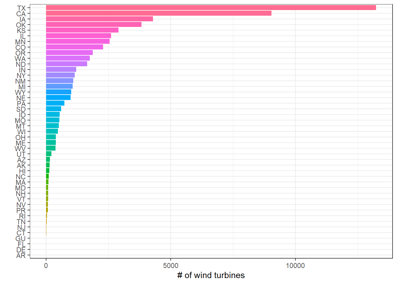
Key turbine metrics faceted by state
state_facet_plot <- function(y, y_title = ""){
  y <- enquo(y)
  wt %>%
    ggplot(aes(p_year, !!y, color = t_state)) +
    geom_point() +
    geom_smooth(method = "lm") +
    facet_geo(~t_state) +
    theme(
      legend.position = "none",
      axis.text.x = element_text(size = 7)
    ) +
    labs(x = "year", y = y_title, title = paste("State-wise", str_to_title(y_title), "Across Time")) +
    scale_x_continuous(n.breaks = 3)
}

state_facet_plot(t_hh, y_title = "turbine hub height (meters)")
state_facet_plot(t_cap, y_title = "turbine capacity (kW)")
state_facet_plot(t_rd, y_title = "turbine rotor diameter (meters)")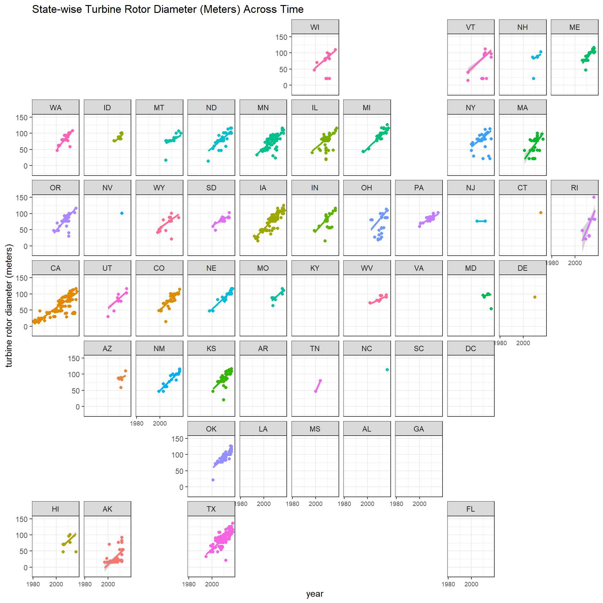
state_facet_plot(t_rsa, y_title = "turbine rotor swept area (meters^2)")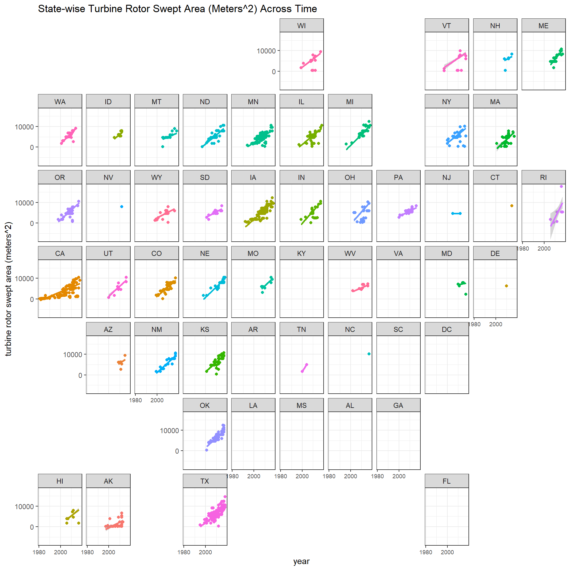
Key combined turbine metrics
metric_plot <- function(y, y_title = ""){
  y <- enquo(y)
  wt %>%
    ggplot(aes(p_year, !!y, color = t_state)) +
    geom_point() +
    geom_smooth(aes(group = 1),method = "lm") +
    theme(
      legend.position = "none"
    ) +
    labs(x = "year", y = y_title, title = paste(str_to_title(y_title), "Across Time"))
}


metric_plot(t_hh, y_title = "turbine hub height (meters)")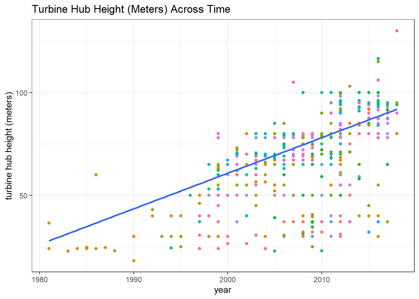
metric_plot(t_cap, y_title = "turbine capacity (kW)")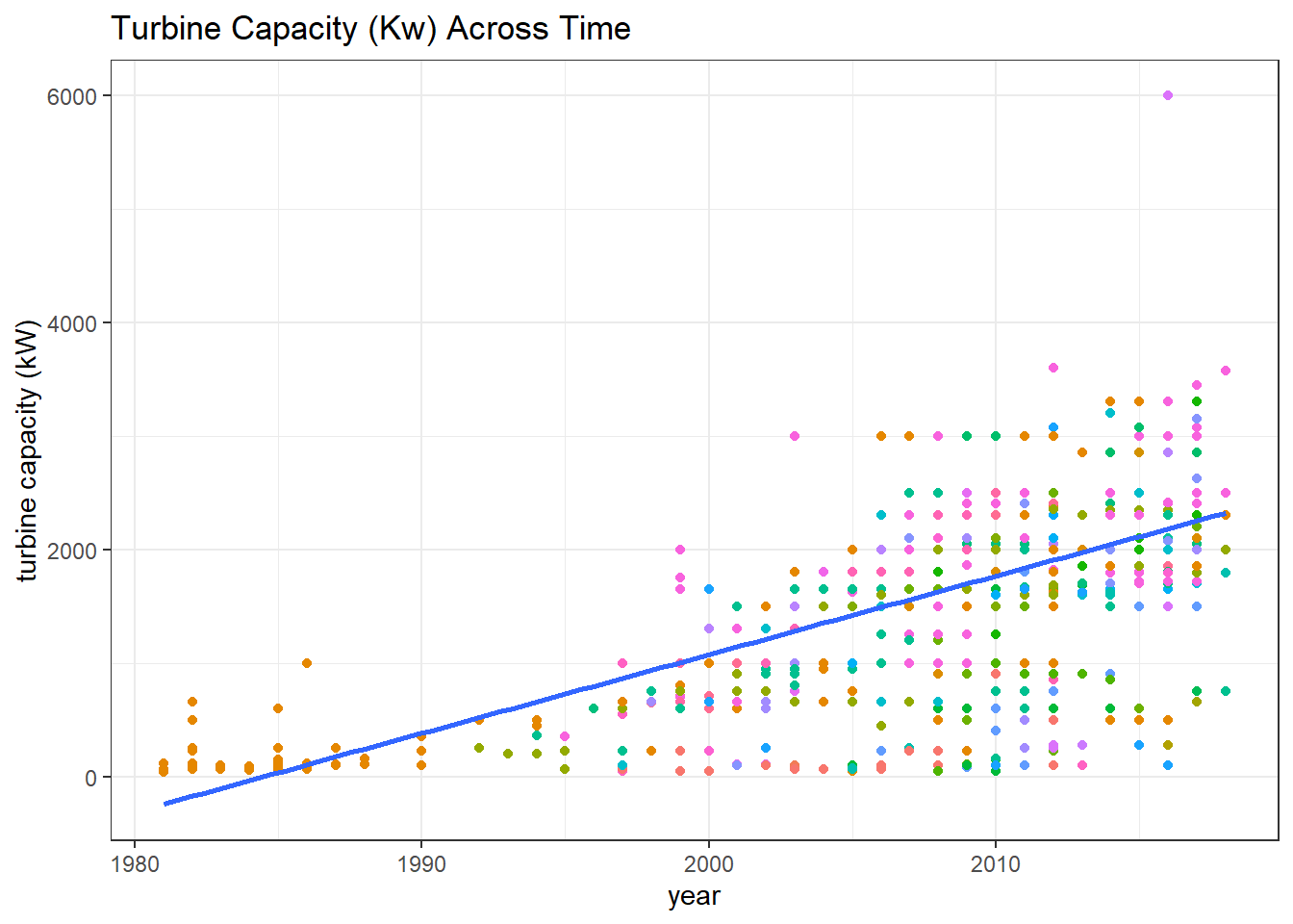
metric_plot(t_rd, y_title = "turbine rotor diameter (meters)")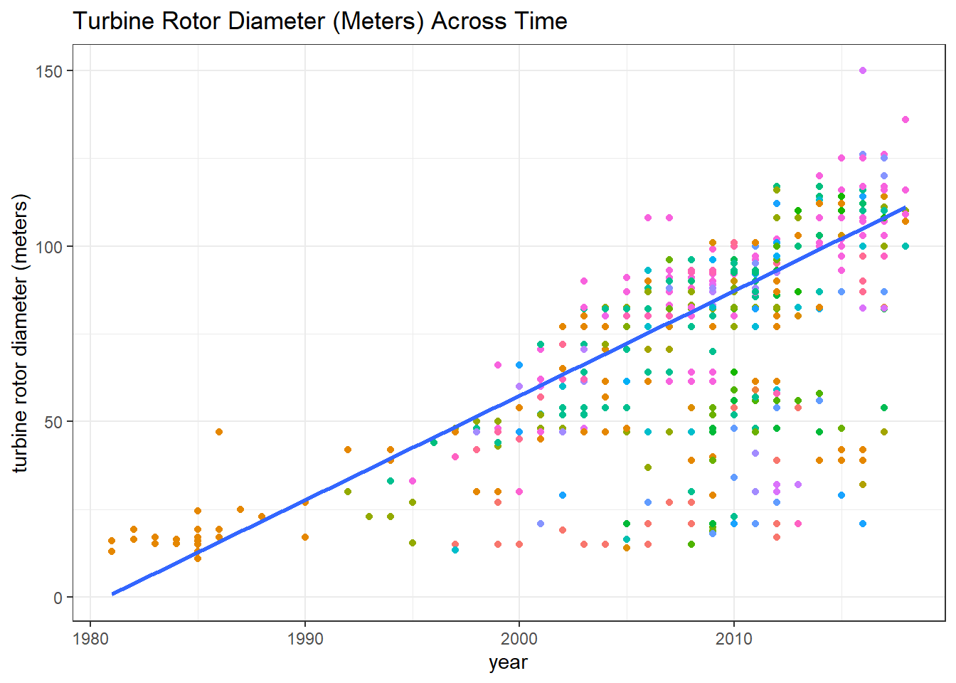
metric_plot(t_rsa, y_title = "turbine rotor swept area (meters^2)")
The U.S. Map with turbine locations
wt %>%
  ggplot(aes(xlong, ylat, color = t_state)) +
    geom_point(show.legend = F) +
    borders("state") +
    coord_map() +
  labs(x = "long", y = "lat", title = "Turbine Locations on the U.S. Map")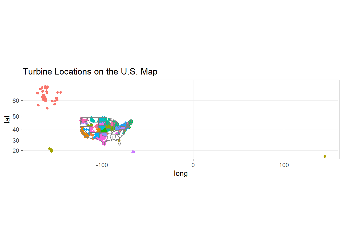
# Removing AK and HI
wt %>%
  filter(xlong < 100 & xlong > -130) %>%
  ggplot(aes(xlong, ylat, color = t_state)) +
    geom_point(show.legend = F) +
    borders("state") +
    coord_map()  +
  labs(x = "long", y = "lat", title = "Turbine Locations on the U.S. Map")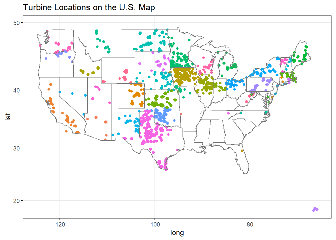
The idea of constructing the following code is inspired by this link.
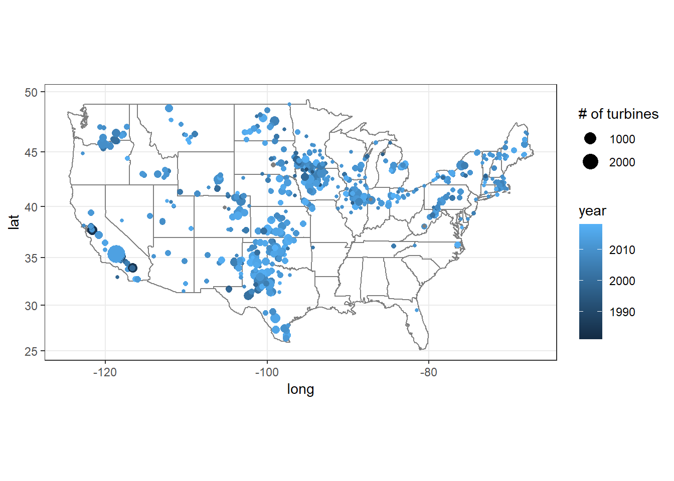
wt %>%
  group_by(t_model, t_state) %>%
  summarize(num_of_turbines = n(),
            long = mean(xlong, na.rm = TRUE),
            lat = mean(ylat, na.rm = TRUE),
            p_year) %>%
  filter(long < 0, long > -130, lat > 20) %>%
  ggplot(aes(long, lat, size = num_of_turbines, color = p_year)) +
  borders("state") +
  geom_point() +
  coord_map() +
  labs(size = "# of turbines", color = "year")
## `summarise()` regrouping output by 't_model', 't_state' (override with `.groups` argument)