Medium Article Text Visualization & LASSO Model
Tue, Sep 14, 2021
7-minute read
This blog post’s data is from TidyTuesday about articles posted on Medium.
library(tidyverse)
library(lubridate)
library(tidytext)
library(widyr)
library(glmnet)
library(broom)
library(ggraph)
library(igraph)
theme_set(theme_bw())
medium <- read_csv("https://raw.githubusercontent.com/rfordatascience/tidytuesday/master/data/2018/2018-12-04/medium_datasci.csv") %>%
mutate(year_month = make_datetime(year = year, month = month, day = day))
head(medium)## # A tibble: 6 x 22
## x1 title subtitle image author publication year month day reading_time
## <dbl> <chr> <chr> <dbl> <chr> <chr> <dbl> <dbl> <dbl> <dbl>
## 1 2 Onlin~ Online a~ 1 Emma ~ NA 2017 8 1 5
## 2 5 A.I. ? NA 0 Sanpa~ NA 2017 8 1 2
## 3 11 Futur~ From Phy~ 1 Z NA 2017 8 1 3
## 4 12 The V~ A true p~ 1 Emiko~ MILLENNIAL~ 2017 8 1 5
## 5 17 Os Me~ mas pera~ 1 Giova~ NEW ORDER 2017 8 1 3
## 6 18 The F~ Original~ 1 Syed ~ Towards Da~ 2017 8 1 6
## # ... with 12 more variables: claps <dbl>, url <chr>, author_url <chr>,
## # tag_ai <dbl>, tag_artificial_intelligence <dbl>, tag_big_data <dbl>,
## # tag_data <dbl>, tag_data_science <dbl>, tag_data_visualization <dbl>,
## # tag_deep_learning <dbl>, tag_machine_learning <dbl>, year_month <dttm>skimr::skim(medium)| Name | medium |
| Number of rows | 78388 |
| Number of columns | 22 |
| _______________________ | |
| Column type frequency: | |
| character | 6 |
| numeric | 15 |
| POSIXct | 1 |
| ________________________ | |
| Group variables | None |
Variable type: character
| skim_variable | n_missing | complete_rate | min | max | empty | n_unique | whitespace |
|---|---|---|---|---|---|---|---|
| title | 1822 | 0.98 | 1 | 230 | 0 | 73953 | 0 |
| subtitle | 30069 | 0.62 | 1 | 362 | 0 | 45838 | 0 |
| author | 286 | 1.00 | 1 | 56 | 0 | 33304 | 0 |
| publication | 44072 | 0.44 | 1 | 133 | 0 | 7297 | 0 |
| url | 0 | 1.00 | 36 | 827 | 0 | 78388 | 0 |
| author_url | 0 | 1.00 | 19 | 68 | 0 | 36006 | 0 |
Variable type: numeric
| skim_variable | n_missing | complete_rate | mean | sd | p0 | p25 | p50 | p75 | p100 | hist |
|---|---|---|---|---|---|---|---|---|---|---|
| x1 | 0 | 1 | 130632.97 | 147899.21 | 0 | 8180.75 | 30598 | 266207.2 | 437504 | ▇▁▁▂▂ |
| image | 0 | 1 | 0.65 | 0.48 | 0 | 0.00 | 1 | 1.0 | 1 | ▅▁▁▁▇ |
| year | 0 | 1 | 2017.66 | 0.47 | 2017 | 2017.00 | 2018 | 2018.0 | 2018 | ▅▁▁▁▇ |
| month | 0 | 1 | 6.21 | 3.31 | 1 | 3.00 | 6 | 9.0 | 12 | ▇▆▆▅▇ |
| day | 0 | 1 | 15.70 | 8.80 | 1 | 8.00 | 16 | 23.0 | 31 | ▇▇▇▇▆ |
| reading_time | 0 | 1 | 4.31 | 3.35 | 0 | 2.00 | 4 | 5.0 | 100 | ▇▁▁▁▁ |
| claps | 0 | 1 | 123.05 | 822.99 | 0 | 0.00 | 4 | 55.0 | 60000 | ▇▁▁▁▁ |
| tag_ai | 0 | 1 | 0.18 | 0.38 | 0 | 0.00 | 0 | 0.0 | 1 | ▇▁▁▁▂ |
| tag_artificial_intelligence | 0 | 1 | 0.38 | 0.48 | 0 | 0.00 | 0 | 1.0 | 1 | ▇▁▁▁▅ |
| tag_big_data | 0 | 1 | 0.11 | 0.31 | 0 | 0.00 | 0 | 0.0 | 1 | ▇▁▁▁▁ |
| tag_data | 0 | 1 | 0.12 | 0.33 | 0 | 0.00 | 0 | 0.0 | 1 | ▇▁▁▁▁ |
| tag_data_science | 0 | 1 | 0.20 | 0.40 | 0 | 0.00 | 0 | 0.0 | 1 | ▇▁▁▁▂ |
| tag_data_visualization | 0 | 1 | 0.06 | 0.23 | 0 | 0.00 | 0 | 0.0 | 1 | ▇▁▁▁▁ |
| tag_deep_learning | 0 | 1 | 0.08 | 0.28 | 0 | 0.00 | 0 | 0.0 | 1 | ▇▁▁▁▁ |
| tag_machine_learning | 0 | 1 | 0.32 | 0.47 | 0 | 0.00 | 0 | 1.0 | 1 | ▇▁▁▁▃ |
Variable type: POSIXct
| skim_variable | n_missing | complete_rate | min | max | median | n_unique |
|---|---|---|---|---|---|---|
| year_month | 0 | 1 | 2017-08-01 | 2018-08-01 | 2018-03-01 | 366 |
Time Series Medium Articles
medium %>%
  group_by(year_month) %>%
  summarize(total = n()) %>%
  ggplot(aes(year_month, total, color = factor(year(year_month)))) +
  geom_point(show.legend = F) +
  geom_smooth(method = "lm") +
  labs(color = NULL, x = NULL, y = "# of articles", title = "# of Medium Articles Along With Time")
Tags
medium_tags <- medium %>%
  pivot_longer(
    cols = starts_with("tag"),
    names_to = "tag",
    values_to = "tag_or_not"
  ) %>%
  mutate(tag = str_remove(tag, pattern = "tag_"))


medium_tags %>%
  group_by(tag) %>%
  summarize(percent = mean(tag_or_not)) %>%
  mutate(tag = fct_reorder(tag, percent)) %>%
  ggplot(aes(percent, tag)) +
  geom_col() +
  scale_x_continuous(labels = scales::percent) +
  labs(x = NULL, title = "Medium Article Tag Percentage") +
  theme(
    axis.text = element_text(size = 13)
  )
medium_tags %>%
  group_by(year = year(year_month), month = month(year_month), tag) %>%
  summarize(avg_tag = mean(tag_or_not)) %>%
  mutate(tag = fct_reorder(tag, avg_tag, .desc = TRUE)) %>%
  ggplot(aes(make_date(year = year, month = month), avg_tag, color = tag)) +
  geom_line(size = 1) +
  scale_y_continuous(labels = scales::percent) +
  labs(x = NULL, y = "Mean Percentage of Articles with Tag",
       title = "Time Series Percentage of Articles with Tag")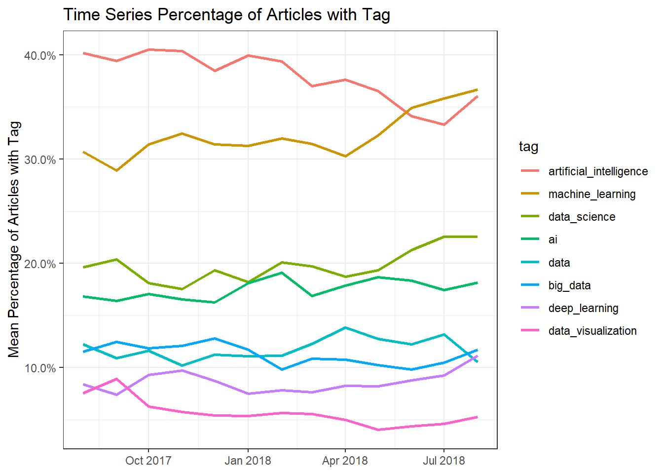
Reading time along with claps
medium_tags %>%
  filter(reading_time <= 60) %>%
  ggplot(aes(factor(reading_time), claps, fill = factor(reading_time))) +
  geom_boxplot() +
  scale_y_log10(labels = scales::comma) +
  coord_flip() +
  theme(
    legend.position = "none"
  ) +
labs(x = "reading time (minutes)", y = "claps (log-scale)", title = "# of Claps with Reading Time") 
Tags with claps
medium_tags %>%
  filter(tag_or_not == 1) %>%
  mutate(tag = fct_reorder(tag, claps, median, na.rm = TRUE)) %>%
  ggplot(aes(tag, claps, fill = tag)) +
  geom_boxplot() +
  scale_y_log10(labels = scales::comma) +
  coord_flip() +
  labs(y = "claps (log10 scale)", title = "Tags and Claps")
Authors with claps
medium_tags %>%
  filter(tag_or_not == 1) %>%
  group_by(author, tag) %>%
  summarize(avg_claps = mean(claps)) %>%
  #arrange(desc(avg_claps)) %>%
  distinct() %>%
  ungroup() %>%
  right_join(medium) %>% View()


top10_authors <- medium_tags %>%
  group_by(author) %>%
  summarize(avg_claps = mean(claps)) %>%
  arrange(desc(avg_claps)) %>%
  head(10) %>%
  select(author) %>%
  pull()

medium_tags %>%
  filter(author %in% top10_authors, tag_or_not == 1) %>%
  count(author, tag, sort = T)
## # A tibble: 15 x 3
## author tag n
## <chr> <chr> <int>
## 1 Fran ois Chollet artificial_intelligence 2
## 2 Andrej Karpathy artificial_intelligence 1
## 3 Andrej Karpathy machine_learning 1
## 4 Anything App ai 1
## 5 Georges Abi-Heila data 1
## 6 Kai Stinchcombe ai 1
## 7 Michael Jordan artificial_intelligence 1
## 8 Michael Jordan data_science 1
## 9 Michael Jordan machine_learning 1
## 10 Radu Raicea artificial_intelligence 1
## 11 Sophia Ciocca artificial_intelligence 1
## 12 Sophia Ciocca machine_learning 1
## 13 Xiaohan Zeng machine_learning 1
## 14 YK Sugi data_science 1
## 15 YK Sugi data_visualization 1Surprisingly, top 10 authors who obtained the largest numbers of claps only have only published at least 2 articles on Medium. That is to say, they might be invited to write something on the platform but are not regular bloggers.
medium_tags %>%
  filter(tag_or_not == 1) %>%
  unnest_tokens(word, title) %>%
  anti_join(stop_words) %>%
  group_by(word) %>%
  summarize(total = n()) %>%
  arrange(desc(total)) %>%
  filter(
    str_detect(word, "[a-z]")
  ) %>%
  head(25) %>%
  mutate(word = fct_reorder(word, total)) %>%
  ggplot(aes(total, word, fill = word)) +
  geom_col(show.legend = F) +
  labs(x = "word count", y = "title word", title = "Top 25 Most Frequent Article Title Words")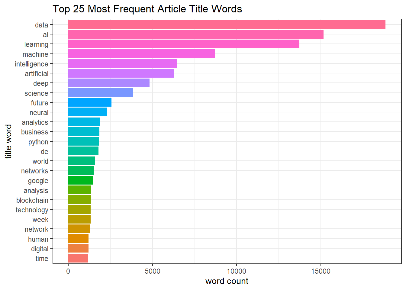
medium_tags %>%
  filter(tag_or_not == 1) %>%
  unnest_tokens(word, subtitle) %>%
  anti_join(stop_words) %>%
  group_by(word) %>%
  summarize(total = n()) %>%
  arrange(desc(total)) %>%
  filter(
    str_detect(word, "[a-z]")
  ) %>%
  head(25) %>%
  mutate(word = fct_reorder(word, total)) %>%
  filter(!is.na(word)) %>%
  ggplot(aes(total, word, fill = word)) +
  geom_col(show.legend = F) +
  labs(x = "word count", y = "subtitle word", title = "Top 25 Most Frequent Article Subtitle Words")
Images and Claps
medium %>%
  mutate(image = factor(image)) %>%
  ggplot(aes(image, claps, fill = image)) +
  geom_boxplot() +
  scale_y_log10(labels = scales::comma) +
  theme(
    legend.position = "none"
  ) +
  labs(x = "contains image or not", y = "# of claps", title = "# of Claps with Whether Articles Containing Image or Not")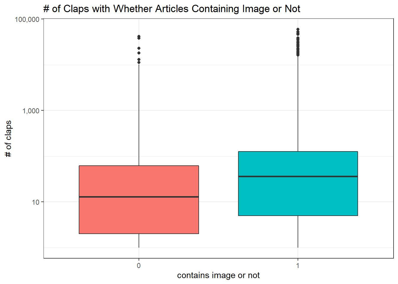
The following graph and LASSO model is adopted from David Robinson’s code with some slight modification.
medium_tags_graph <- medium_tags %>%
  filter(tag_or_not == 1) %>%
  mutate(article_id = row_number()) %>%
  select(title, tag, article_id, claps) %>%
  unnest_tokens(word, title) %>%
  anti_join(stop_words) %>%
  add_count(word) %>%
  filter(n > 500, str_detect(word, "[a-z]"))

word_cor <- medium_tags_graph %>%
  pairwise_cor(word, article_id, sort = TRUE)

vertices <- medium_tags_graph %>%
  group_by(word) %>%
  summarize(median_claps = median(claps),
            geometric_mean_claps = exp(mean(log(claps + 1))) - 1,
            occurences = n()) %>%
  arrange(desc(median_claps)) %>%
  filter(word %in% word_cor$item1 |
         word %in% word_cor$item2)

word_cor %>%
  head(50) %>%
  graph_from_data_frame(vertices = vertices) %>%
  ggraph(layout = "fr") +
  geom_edge_link() +
  geom_node_point(aes(size = occurences,
                      color = geometric_mean_claps)) +
  geom_node_text(aes(label = name), repel = TRUE) +
  scale_color_gradient2(low = "red", high = "blue", midpoint = 20) +
  theme_void() +
  labs(title = "Claps with Titles",
       subtitle = "Color shows the geometric mean of # of claps on articles with this word in the title",
       size = "# of occurrences",
       color = "claps")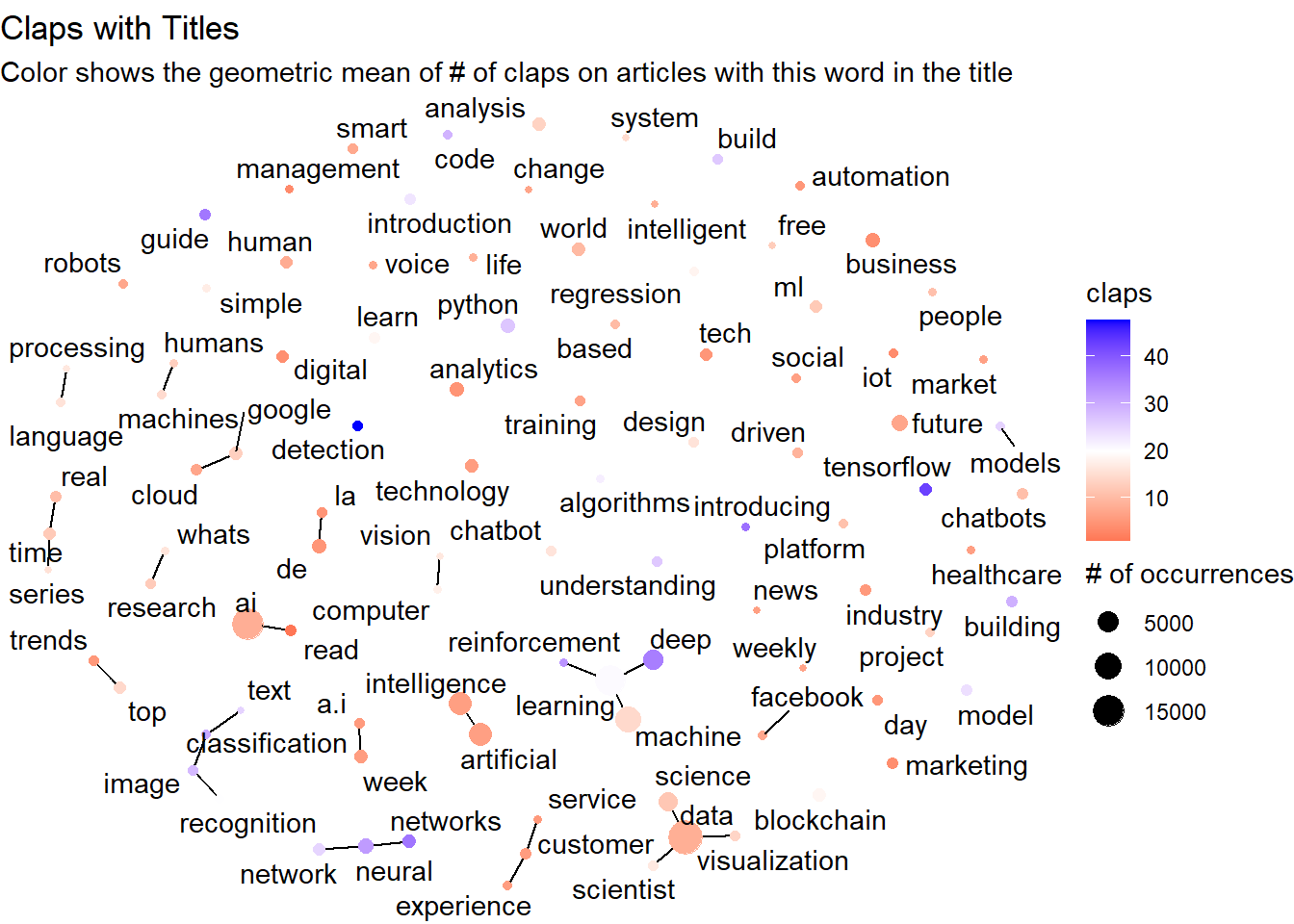
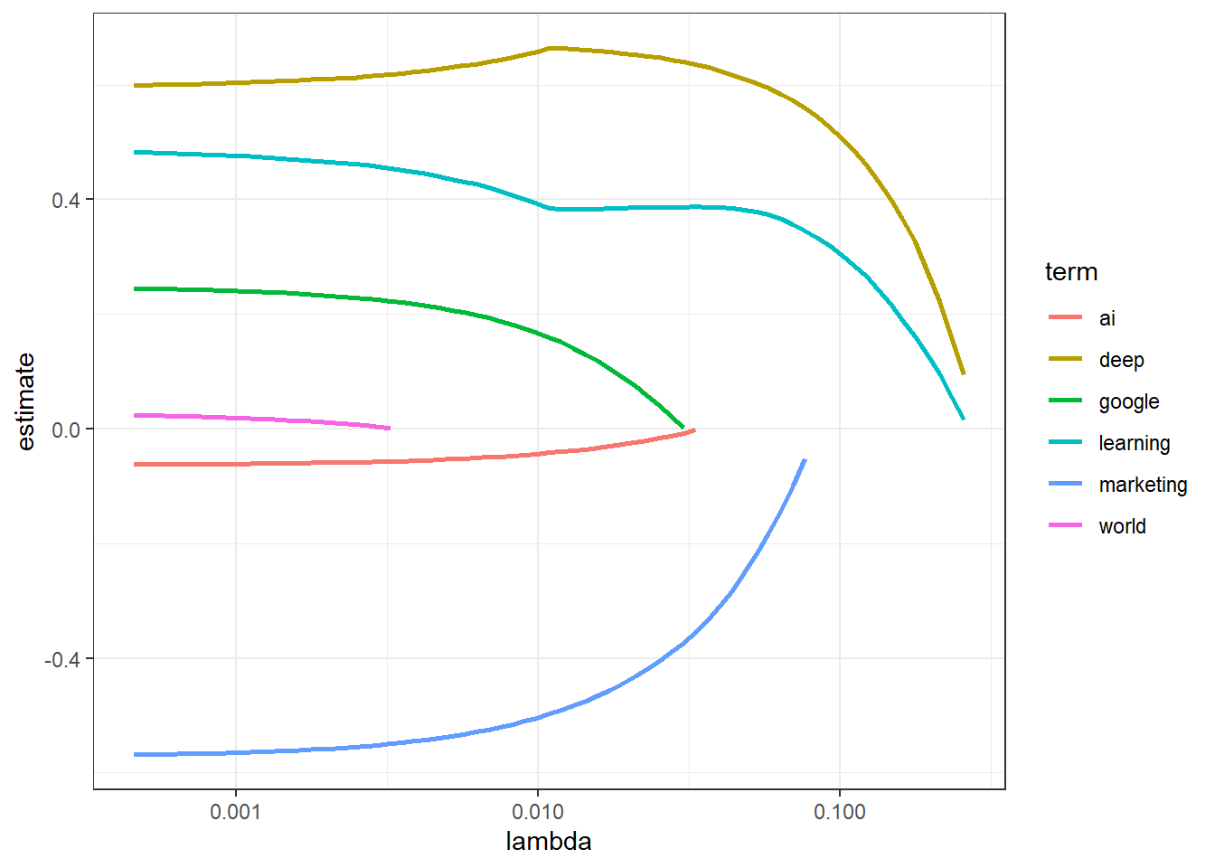
LASSO Model
sparse_matrix <- medium_tags_graph %>%
  distinct(article_id, word, claps) %>%
  cast_sparse(article_id, word)

claps <- medium_tags_graph$claps[match(rownames(sparse_matrix), as.character(medium_tags_graph$article_id))]

lasso_model <- cv.glmnet(sparse_matrix, log(claps + 1))

tidy(lasso_model$glmnet.fit) %>%
  filter(term %in% c("ai", "learning", "world", "deep", "google", "marketing")) %>%
  ggplot(aes(lambda, estimate, color = term)) +
  geom_line(size = 1) +
  scale_x_log10()