NYC Restaurants Visualization & PCA
Thu, Sep 16, 2021
7-minute read
This blog post analyzes the dataset about the inspections on the restaurants in NYC, and the dataset is obtained from TidyTuesday.
library(tidyverse)
library(lubridate)
library(scales)
library(ggthemes)
library(widyr)
library(broom)
theme_set(theme_tufte())
nyr <- read_csv("https://data.cityofnewyork.us/api/views/43nn-pn8j/rows.csv") %>%
janitor::clean_names() %>%
select(-phone, -grade_date, -record_date, -building, -street) %>%
mutate(inspection_date = mdy(inspection_date),
cuisine_description = case_when(
cuisine_description == "Latin (Cuban, Dominican, Puerto Rican, South & Central American)" ~ "Latin",
TRUE ~ as.character(cuisine_description)
)) %>%
filter(inspection_date > 2000)
nyr## # A tibble: 378,107 x 21
## camis dba boro zipcode cuisine_descript~ inspection_date action
## <dbl> <chr> <chr> <dbl> <chr> <date> <chr>
## 1 41636061 JACK'S ~ Manha~ 10012 American 2017-06-26 Violation~
## 2 50045844 HOT SPO~ Brook~ 11204 Chinese/Japanese 2017-04-05 Violation~
## 3 41521159 CITY SA~ Manha~ 10036 Sandwiches/Salad~ 2019-06-19 Violation~
## 4 41576944 TRIX Brook~ 11211 French 2017-01-27 Violation~
## 5 50003506 LUPITA ~ Manha~ 10029 Mexican 2017-10-25 Violation~
## 6 50098012 FRIENDL~ Brook~ 11206 Sandwiches/Salad~ 2021-08-23 Violation~
## 7 50051744 ORCHARD~ Bronx 10464 Coffee/Tea 2016-08-17 Violation~
## 8 50008223 SUBWAY Bronx 10457 Sandwiches 2019-05-10 Violation~
## 9 41694845 THE WIC~ Brook~ 11209 American 2021-08-17 Violation~
## 10 41694845 THE WIC~ Brook~ 11209 American 2021-08-17 Violation~
## # ... with 378,097 more rows, and 14 more variables: violation_code <chr>,
## # violation_description <chr>, critical_flag <chr>, score <dbl>, grade <chr>,
## # inspection_type <chr>, latitude <dbl>, longitude <dbl>,
## # community_board <dbl>, council_district <chr>, census_tract <chr>,
## # bin <dbl>, bbl <dbl>, nta <chr>nyr <- nyr %>%
separate(inspection_type, c("inspection_program", "inspection_type"), sep = " / ") skimr::skim(nyr)| Name | nyr |
| Number of rows | 378107 |
| Number of columns | 22 |
| _______________________ | |
| Column type frequency: | |
| character | 13 |
| Date | 1 |
| numeric | 8 |
| ________________________ | |
| Group variables | None |
Variable type: character
| skim_variable | n_missing | complete_rate | min | max | empty | n_unique | whitespace |
|---|---|---|---|---|---|---|---|
| dba | 56 | 1.00 | 2 | 90 | 0 | 20072 | 0 |
| boro | 0 | 1.00 | 1 | 13 | 0 | 6 | 0 |
| cuisine_description | 1 | 1.00 | 4 | 30 | 0 | 85 | 0 |
| action | 0 | 1.00 | 33 | 130 | 0 | 5 | 0 |
| violation_code | 4652 | 0.99 | 3 | 4 | 0 | 106 | 0 |
| violation_description | 2217 | 0.99 | 19 | 360 | 0 | 106 | 0 |
| critical_flag | 0 | 1.00 | 8 | 14 | 0 | 3 | 0 |
| grade | 184964 | 0.51 | 1 | 1 | 0 | 7 | 0 |
| inspection_program | 0 | 1.00 | 9 | 28 | 0 | 8 | 0 |
| inspection_type | 0 | 1.00 | 13 | 28 | 0 | 6 | 0 |
| council_district | 6626 | 0.98 | 2 | 2 | 0 | 51 | 0 |
| census_tract | 6626 | 0.98 | 6 | 6 | 0 | 1178 | 0 |
| nta | 6626 | 0.98 | 4 | 4 | 0 | 193 | 0 |
Variable type: Date
| skim_variable | n_missing | complete_rate | min | max | median | n_unique |
|---|---|---|---|---|---|---|
| inspection_date | 0 | 1 | 2009-06-22 | 2021-09-16 | 2019-01-22 | 1486 |
Variable type: numeric
| skim_variable | n_missing | complete_rate | mean | sd | p0 | p25 | p50 | p75 | p100 | hist |
|---|---|---|---|---|---|---|---|---|---|---|
| camis | 0 | 1.00 | 46363746.72 | 4.369762e+06 | 30075445.00 | 41428295.00 | 50011515.00 | 50061285.00 | 5.011492e+07 | ▁▁▆▁▇ |
| zipcode | 5624 | 0.99 | 10681.84 | 6.019200e+02 | 10000.00 | 10022.00 | 10469.00 | 11229.00 | 3.033900e+04 | ▇▁▁▁▁ |
| score | 13539 | 0.96 | 20.35 | 1.490000e+01 | 0.00 | 11.00 | 15.00 | 26.00 | 1.640000e+02 | ▇▂▁▁▁ |
| latitude | 353 | 1.00 | 40.12 | 4.930000e+00 | 0.00 | 40.69 | 40.73 | 40.76 | 4.091000e+01 | ▁▁▁▁▇ |
| longitude | 353 | 1.00 | -72.84 | 8.940000e+00 | -74.25 | -73.99 | -73.96 | -73.90 | 0.000000e+00 | ▇▁▁▁▁ |
| community_board | 6626 | 0.98 | 248.49 | 1.301500e+02 | 101.00 | 105.00 | 301.00 | 401.00 | 5.950000e+02 | ▇▂▅▅▁ |
| bin | 8344 | 0.98 | 2510375.18 | 1.346132e+06 | 1000000.00 | 1043896.00 | 3007533.00 | 4002366.00 | 5.799501e+06 | ▇▂▅▅▁ |
| bbl | 1015 | 1.00 | 2400511137.26 | 1.339002e+09 | 1.00 | 1010420121.00 | 3001670003.00 | 4001630004.00 | 5.270001e+09 | ▇▂▅▅▁ |
Total # of Cuisine counts
nyr %>%
  filter(!is.na(cuisine_description)) %>%
  count(cuisine_description, sort = T) %>%
  mutate(cuisine_description = fct_lump(cuisine_description, n = 10, w = n),
         cuisine_description = fct_reorder(cuisine_description, n)) %>%
  ggplot(aes(n, cuisine_description)) +
  geom_col() +
  labs(x = "# of restaurants", y = "cuisine", title = "NYC Cuisine #")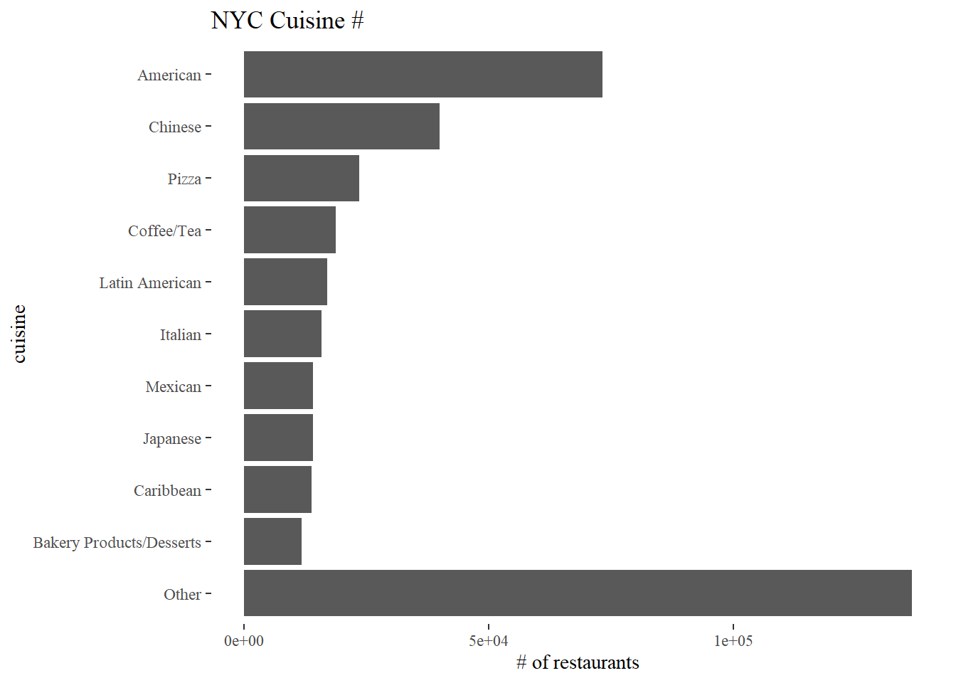
Top 10 Cuisines and their critical flag counts
top_10_cuisines <- nyr %>%
  count(cuisine_description, sort = T) %>%
  head(10) %>%
  select(cuisine_description) %>%
  pull()

nyr_top10 <- nyr %>%
  filter(cuisine_description %in% top_10_cuisines,
         critical_flag != "Not Applicable")

nyr_top10 %>%
  count(cuisine_description, critical_flag, sort = T) %>%
  ggplot(aes(n, cuisine_description)) +
  geom_col() +
  facet_wrap(~critical_flag) +
  labs(x = "# of restaurants", y = "cuisine",
       title = "Top 10 Cuisine and Their Critical Flag Counts")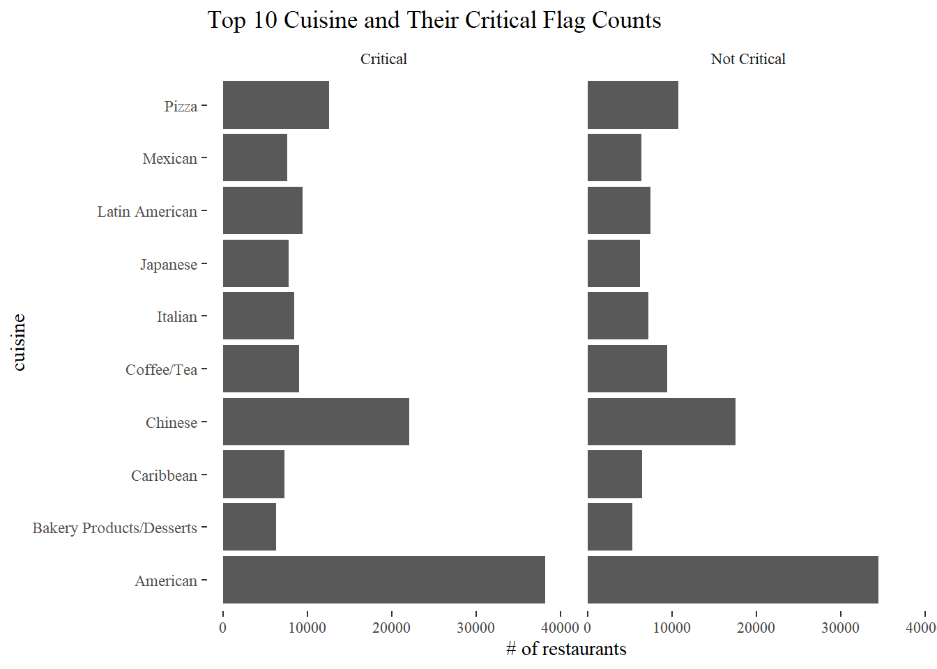
Top 10 Cuisine and their critical flag percentage
total_restaurants <- nyr %>%
  filter(cuisine_description %in% top_10_cuisines) %>%
  group_by(cuisine_description) %>%
  summarize(total = n())

nyr_top10 %>%
  left_join(total_restaurants) %>%
  group_by(cuisine_description, critical_flag) %>%
  summarize(critical_percentage = n()/total) %>%
  distinct() %>%
  ggplot(aes(critical_percentage, cuisine_description)) +
  geom_col() +
  facet_wrap(~critical_flag) +
  expand_limits(x = 1) +
  scale_x_continuous(labels = percent) +
  labs(x = "percentage", y = "cuisine",
       title = "Top 10 Cuisine and Their Critical Flag Percentage")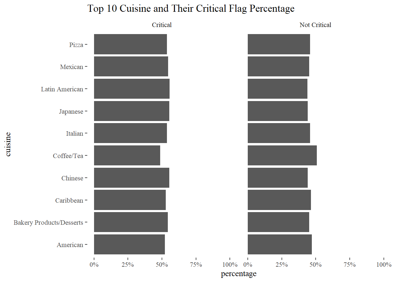
Grades and inspection date
nyr %>%
  filter(year(inspection_date) > 2016,
         !is.na(grade),
         !boro %in% c("Missing", 0),
         !grade %in% c("Not Yet Graded", "G")) %>%
  count(grade, inspection_date, boro) %>%
  ggplot(aes(inspection_date, n, fill = grade)) +
  geom_area(show.legend = F) +
  theme(
    axis.text.x = element_text(angle = 90)
  ) +
  facet_grid(boro~grade) +
  labs(x = "inspection date", y = "# of restaurants",
       title = "Inspection Date and Grades")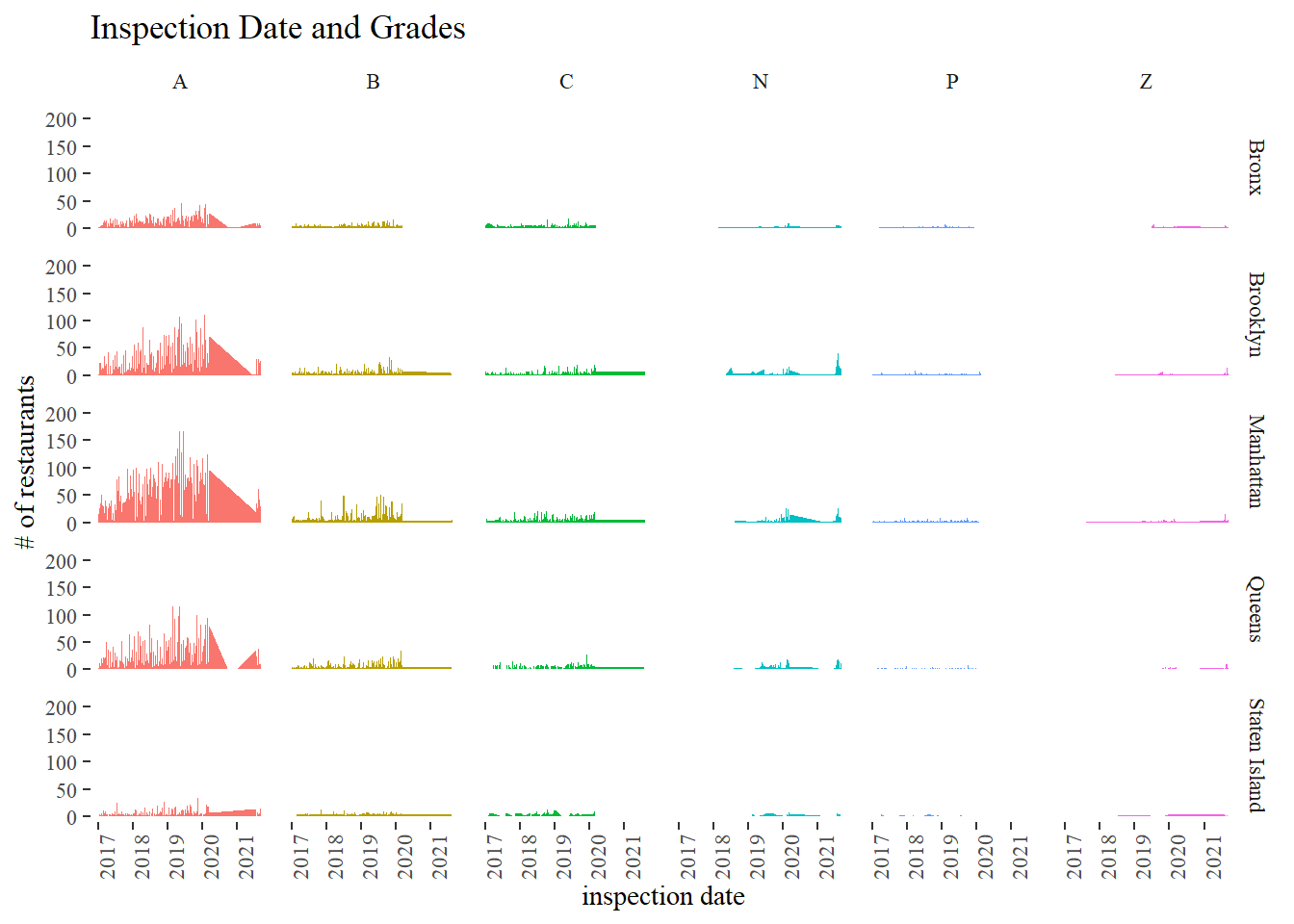
Boro and critical flags
nyr %>%
  mutate(year = year(inspection_date)) %>%
  filter(year > 2015,
         boro != 0) %>%
  count(year, boro, critical_flag, sort = T) %>%
  ggplot(aes(critical_flag, boro, fill = n)) +
  geom_tile() +
  facet_wrap(~year, ncol = 1) +
  scale_fill_gradient2(
    low = "blue",
    high = "red",
    mid = "white",
    midpoint = 10000
  ) +
  labs(x = "Critical Flag", y = NULL, fill = "# of restaurants",
       title = "Yearly Critical Flags among All 5 Boros in NYC")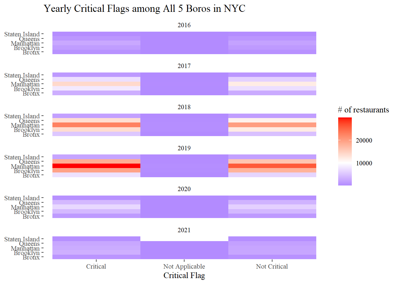
There is no the same camis that changed its name based on dba.
nyr %>%
  count(camis, dba, sort = T) %>%
  count(camis, sort = T)
## # A tibble: 25,022 x 2
## camis n
## <dbl> <int>
## 1 30075445 1
## 2 30112340 1
## 3 30191841 1
## 4 40356018 1
## 5 40356483 1
## 6 40356731 1
## 7 40357217 1
## 8 40359480 1
## 9 40359705 1
## 10 40360045 1
## # ... with 25,012 more rowsInspection Type and critical flag
nyr %>%
  filter(boro != 0,
         critical_flag != "Not Critical") %>%
  count(critical_flag, inspection_type, boro) %>%
  ggplot(aes(critical_flag, inspection_type, fill = n)) +
  geom_tile() +
  facet_wrap(~boro) +
  scale_fill_gradient2(
    low = "blue",
    high = "red",
    mid = "white",
    midpoint = 10000
  ) +
  labs(x = "Critical Flag", y = "Inspection Type", fill = "# of restaurants",
       title = "Inspection Types and Critical Flags among All Boros in NYC")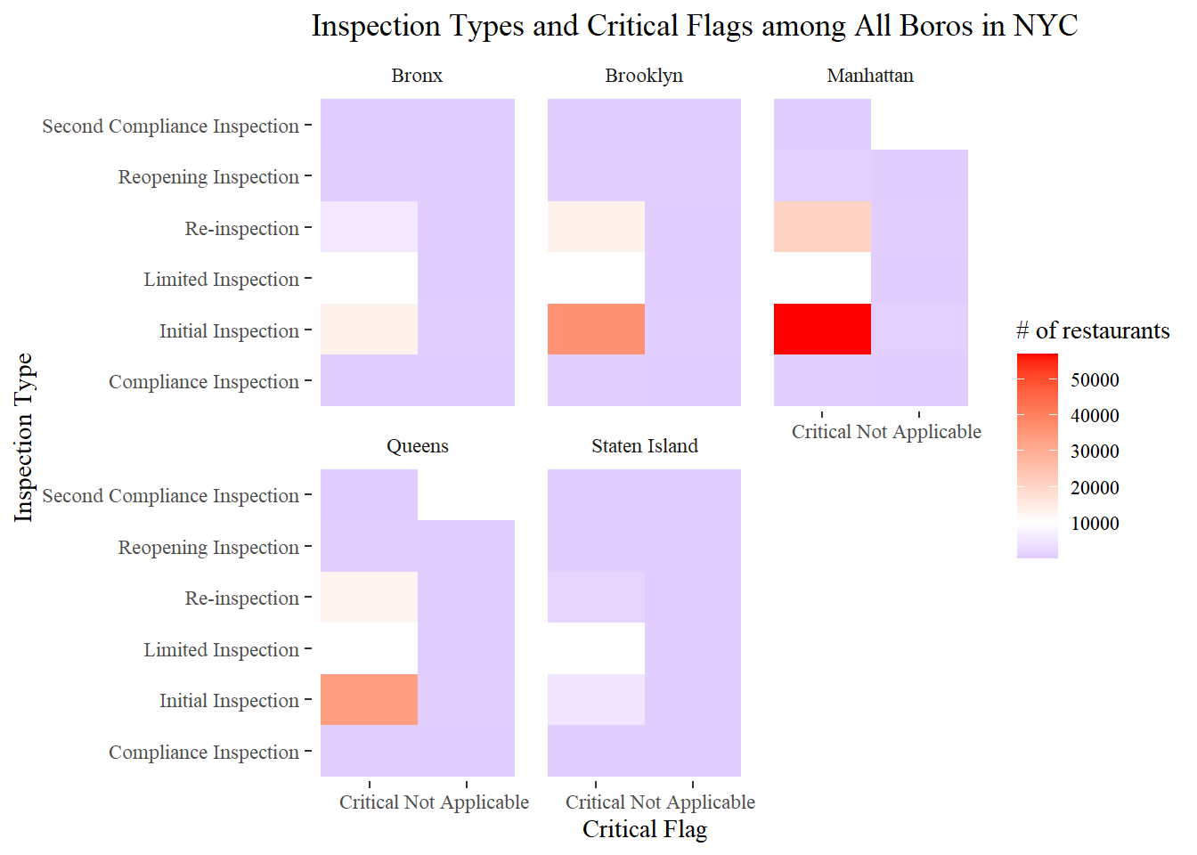
The following code is inspired by David Robinson’s code for learning purposes only, but some chunks of code do not work for some reason.
inspections <- nyr %>%
  group_by(camis,
           dba,
           boro,
           zipcode,
           cuisine_description,
           inspection_date,
           action,
           score,
           grade,
           inspection_type,
           inspection_program) %>%
  summarize(
    critical_violations = sum(critical_flag == "Critical"),
    non_critical_violations = sum(critical_flag == "Not Critical")
  ) %>%
  ungroup()


most_recent_cycle_inspection <- inspections %>%
  filter(inspection_program == "Cycle Inspection",
         inspection_type == "Initial Inspection") %>%
  arrange(desc(inspection_date)) %>%
  distinct(camis, .keep_all = TRUE)
by_dba <- most_recent_cycle_inspection %>%
group_by(dba, cuisine = cuisine_description) %>%
summarize(locations = n(),
avg_score = mean(score),
median_score = median(score)) %>%
ungroup() %>%
arrange(desc(locations))## `summarise()` has grouped output by 'dba'. You can override using the `.groups` argument.by_dba %>%
mutate(locations_bin = cut(locations, c(0, 1, 3, 10, Inf), labels = c("1", "2-3", "4-10", ">10"))) %>%
ggplot(aes(locations_bin, avg_score + 1, fill = locations_bin)) +
geom_boxplot(show.legend = F) +
scale_y_log10() +
labs(x = "# of location(s)", y = "Average Score (+1)",
title = "Relation Between # of Locations & Average Score")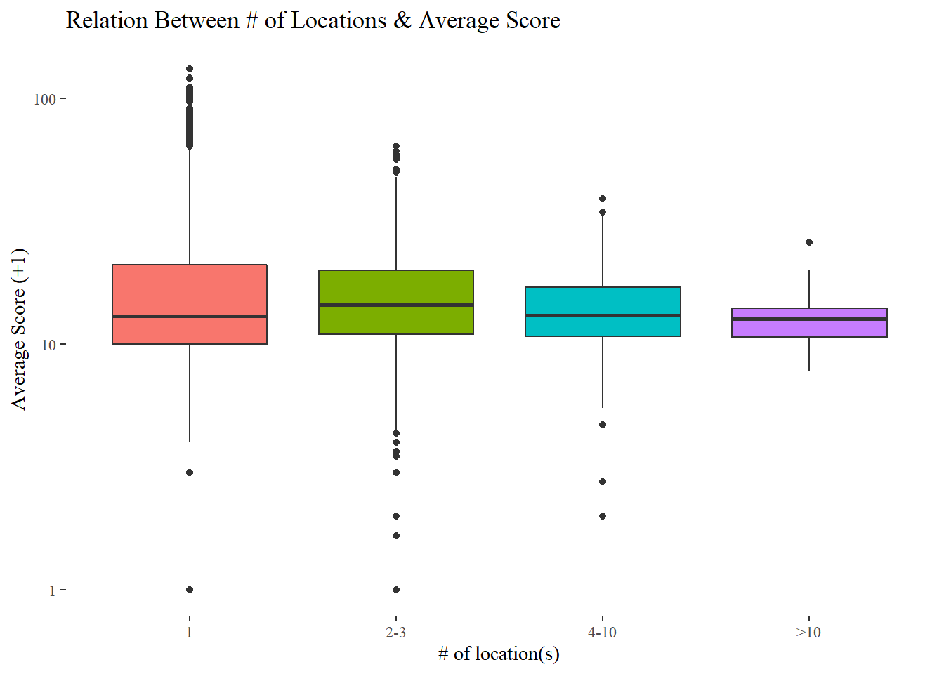
For some unknown reason, David’s code strangely does not work, and here is the updated one that works. Note: The original code is commented out.
by_dba %>%
  add_count(cuisine) %>%
  filter(n > 200) %>%
  nest(-cuisine) %>%
  mutate(model = map(data, ~ t.test(.$avg_score)),
         tidied = map(model, tidy)) %>%
  #unnest(map(model, tidy))
  #mutate(tidied = map(model, tidy)) %>%
  unnest(tidied) %>%
  mutate(
    cuisine = fct_reorder(cuisine, estimate)
  ) %>%
  ggplot(aes(estimate, cuisine)) +
  geom_point() +
  geom_errorbar(aes(xmin = conf.low,
                    xmax = conf.high)) +
  labs(x = "estimated average score",
       title = "Estimated Average Score with Confidence Interval")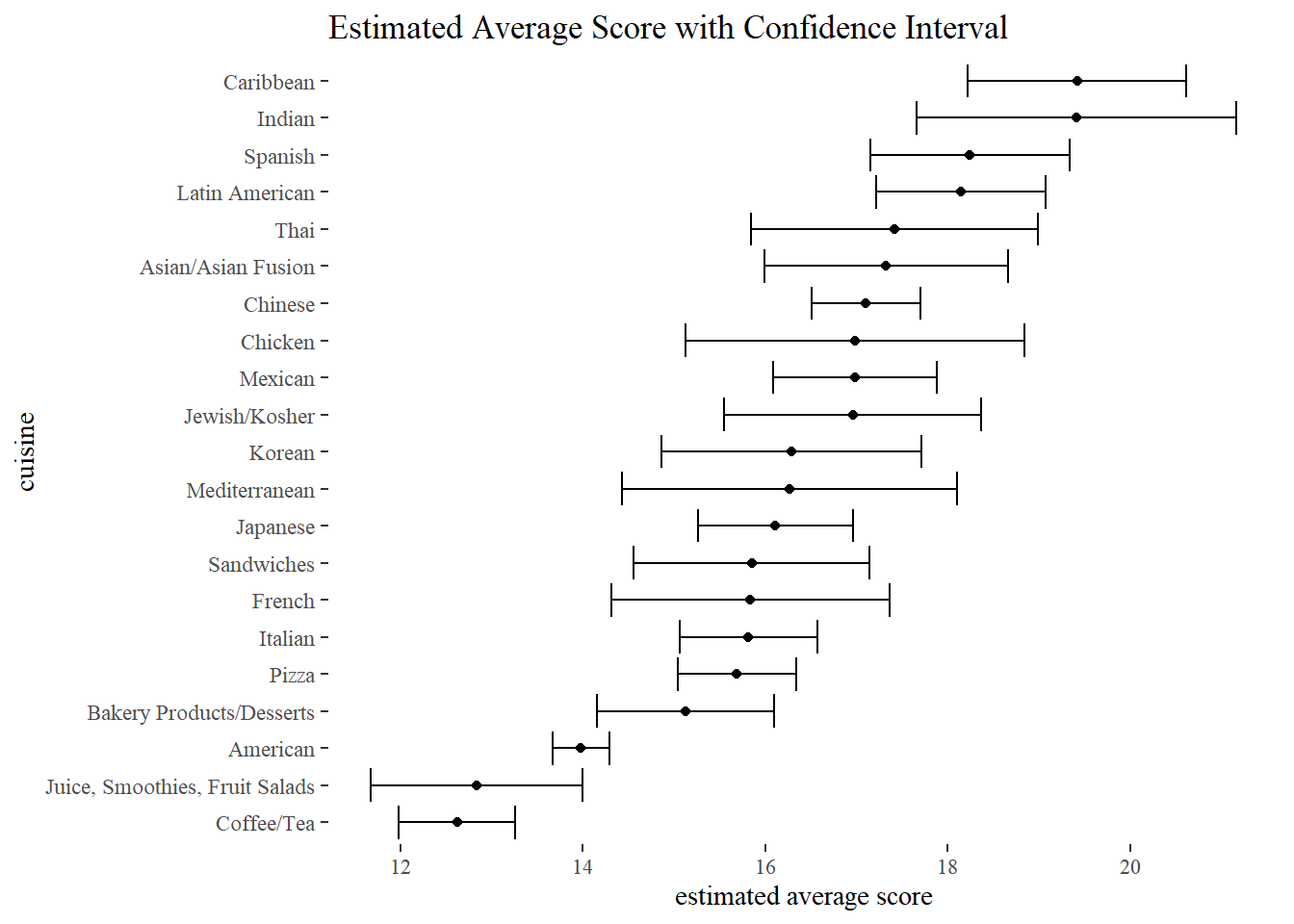
violations <- nyr %>%
  semi_join(most_recent_cycle_inspection, by = c("camis", "inspection_date")) %>%
  filter(!is.na(violation_description))

violations %>%
  pairwise_cor(violation_description, camis, sort = TRUE)
## # A tibble: 7,310 x 3
## item1 item2 correlation
## <chr> <chr> <dbl>
## 1 Food not labeled in accordance ~ Records and logs not maintained~ 0.866
## 2 Records and logs not maintained~ Food not labeled in accordance ~ 0.866
## 3 Required nutritional informatio~ Additional nutritional informat~ 0.764
## 4 Additional nutritional informat~ Required nutritional informatio~ 0.764
## 5 ROP processing equipment not ap~ HACCP plan not approved or appr~ 0.750
## 6 HACCP plan not approved or appr~ ROP processing equipment not ap~ 0.750
## 7 Facility not vermin proof. Harb~ Evidence of mice or live mice p~ 0.625
## 8 Evidence of mice or live mice p~ Facility not vermin proof. Harb~ 0.625
## 9 Filth flies or food/refuse/sewa~ Facility not vermin proof. Harb~ 0.532
## 10 Facility not vermin proof. Harb~ Filth flies or food/refuse/sewa~ 0.532
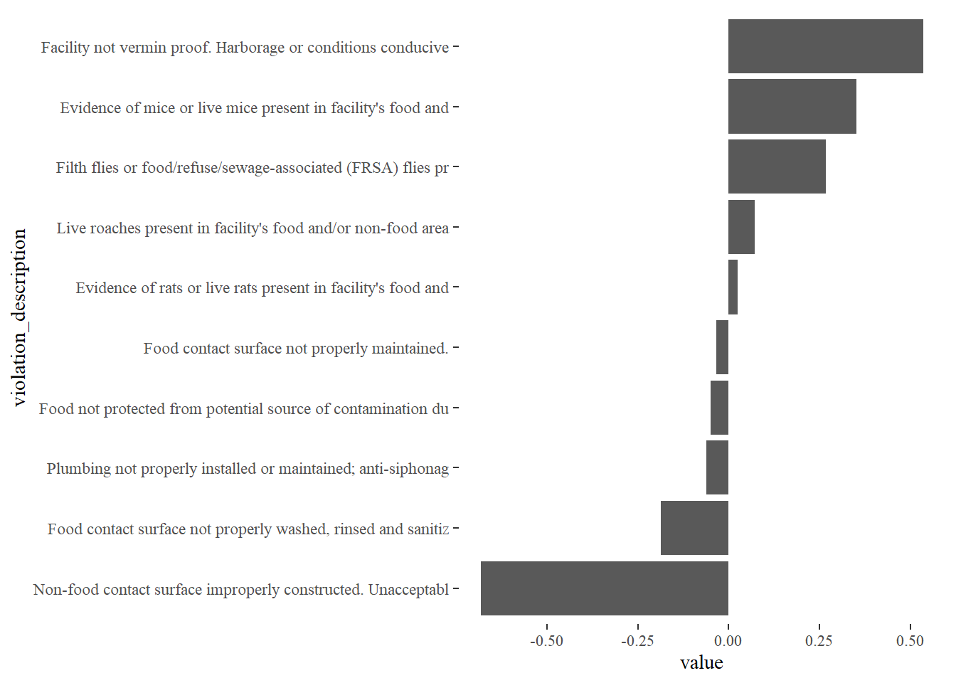
## # ... with 7,300 more rowsPCA
principal_components <- violations %>%
  mutate(value = 1) %>%
  widely_svd(violation_description, camis, value, nv = 6)

principal_components %>%
  filter(dimension == 2) %>%
  top_n(10, abs(value)) %>%
  mutate(violation_description = str_sub(violation_description, 1, 60),
         violation_description = fct_reorder(violation_description, value)) %>%
  ggplot(aes(violation_description, value)) +
  geom_col() +
  coord_flip()