Dolphin Data Visualization & Survival Analysis (with fuzzyjoin package used)
Fri, Sep 17, 2021
6-minute read
The dataset of this blog post is from TidyTuesday about whales and dolphins in the US between 1938 and 2017.
library(tidyverse)
library(scales)
library(lubridate)
library(fuzzyjoin)
library(broom)
library(survival)
theme_set(theme_bw())
dolphins <- read_csv("https://raw.githubusercontent.com/rfordatascience/tidytuesday/master/data/2018/2018-12-18/allCetaceanData.csv") %>%
select(-X1) %>%
mutate(sex = case_when(
sex == "F" ~ "Female",
sex == "M" ~ "Male",
sex == "U" ~ "Unkown",
TRUE ~ as.character(sex)
),
birthYear = as.numeric(birthYear))
dolphins## # A tibble: 2,194 x 21
## species id name sex accuracy birthYear acquisition originDate
## <chr> <chr> <chr> <chr> <chr> <dbl> <chr> <date>
## 1 Bottlenose NOA0004614,~ Dazz~ Fema~ a 1989 Born 1989-04-07
## 2 Bottlenose NOA0004386,~ Tursi Fema~ a 1973 Born 1973-11-26
## 3 Bottlenose NOA0002137,~ Star~ Male a 1978 Born 1978-05-13
## 4 Bottlenose NOA0002690,~ Sandy Fema~ a 1979 Born 1979-02-03
## 5 Bottlenose NOA0004418,~ Sandy Male a 1979 Born 1979-08-15
## 6 Bottlenose NOA0002725,~ Nacha Fema~ a 1980 Born 1980-10-10
## 7 Bottlenose NOA0005036,~ Kama Male a 1981 Born 1981-03-27
## 8 Bottlenose NOA0002746,~ Jene~ Fema~ a 1981 Born 1981-10-20
## 9 Bottlenose NOA0002766,~ Duffy Male a 1982 Born 1982-10-16
## 10 Bottlenose NOA0002784,~ Astra Fema~ a 1983 Born 1983-03-07
## # ... with 2,184 more rows, and 13 more variables: originLocation <chr>,
## # mother <chr>, father <chr>, transfers <chr>, currently <chr>, region <chr>,
## # status <chr>, statusDate <date>, COD <chr>, notes <chr>,
## # transferDate <date>, transfer <chr>, entryDate <date>skimr::skim(dolphins)| Name | dolphins |
| Number of rows | 2194 |
| Number of columns | 21 |
| _______________________ | |
| Column type frequency: | |
| character | 16 |
| Date | 4 |
| numeric | 1 |
| ________________________ | |
| Group variables | None |
Variable type: character
| skim_variable | n_missing | complete_rate | min | max | empty | n_unique | whitespace |
|---|---|---|---|---|---|---|---|
| species | 0 | 1.00 | 6 | 24 | 0 | 37 | 0 |
| id | 0 | 1.00 | 3 | 88 | 0 | 2161 | 0 |
| name | 448 | 0.80 | 1 | 18 | 0 | 1364 | 0 |
| sex | 0 | 1.00 | 4 | 6 | 0 | 3 | 0 |
| accuracy | 0 | 1.00 | 1 | 1 | 0 | 3 | 0 |
| acquisition | 0 | 1.00 | 4 | 11 | 0 | 6 | 0 |
| originLocation | 0 | 1.00 | 7 | 27 | 0 | 121 | 0 |
| mother | 1606 | 0.27 | 2 | 20 | 0 | 233 | 0 |
| father | 1710 | 0.22 | 1 | 26 | 0 | 150 | 0 |
| transfers | 1392 | 0.37 | 36 | 508 | 0 | 632 | 0 |
| currently | 0 | 1.00 | 7 | 42 | 0 | 97 | 0 |
| region | 0 | 1.00 | 2 | 2 | 0 | 1 | 0 |
| status | 0 | 1.00 | 4 | 20 | 0 | 9 | 0 |
| COD | 669 | 0.70 | 1 | 137 | 0 | 1002 | 0 |
| notes | 1975 | 0.10 | 9 | 306 | 0 | 164 | 0 |
| transfer | 0 | 1.00 | 2 | 7 | 0 | 2 | 0 |
Variable type: Date
| skim_variable | n_missing | complete_rate | min | max | median | n_unique |
|---|---|---|---|---|---|---|
| originDate | 69 | 0.97 | 1946-01-01 | 2017-04-19 | 1983-03-28 | 1459 |
| statusDate | 534 | 0.76 | 1962-09-22 | 2017-01-31 | 1986-10-07 | 1416 |
| transferDate | 2173 | 0.01 | 1980-04-23 | 2011-04-17 | 2005-10-17 | 14 |
| entryDate | 70 | 0.97 | 1946-01-01 | 2017-04-19 | 1983-06-18 | 1458 |
Variable type: numeric
| skim_variable | n_missing | complete_rate | mean | sd | p0 | p25 | p50 | p75 | p100 | hist |
|---|---|---|---|---|---|---|---|---|---|---|
| birthYear | 694 | 0.68 | 1985.43 | 16.7 | 1938 | 1972 | 1984 | 2000 | 2017 | ▁▅▇▅▅ |
Top 5 Species Faceted by Sex
dolphins %>%
  count(species, sex, sort = T) %>%
  mutate(species = str_remove(species, "[,;].+"),
         species = fct_lump(species, n = 5, w = n),
         species = fct_reorder(species, n)
         ) %>%
  ggplot(aes(n, species, fill = species)) +
  geom_col(show.legend = F) +
  facet_wrap(~sex) +
  theme(
    strip.text = element_text(size = 10, face = "bold")
  ) +
  labs(x = "# of dolphins",
       title = "Top 5 Species Faceted by Sex")
dolphins %>%
  count(birthYear, sex, sort = T) %>%
  filter(!is.na(birthYear)) %>%
  ggplot(aes(birthYear, n, color = sex)) +
  geom_line(size = 1) +
  facet_wrap(~sex, ncol = 1) +
  theme(
    strip.text = element_text(size = 10, face = "bold")
  ) +
  labs(color = NULL,
       x = "birth year",
       y = "# of dolphins born",
       title = "Yearly Birth Counts") +
  scale_x_continuous(breaks = seq(1940, 2020, by = 10))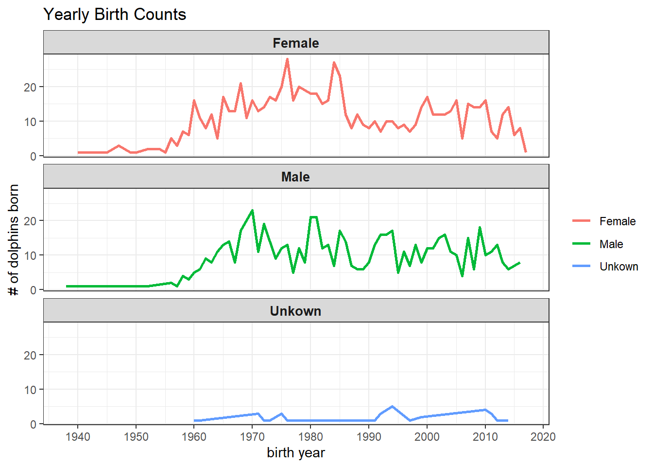
Birth year distribution
dolphins %>%
  ggplot(aes(birthYear)) +
geom_histogram() 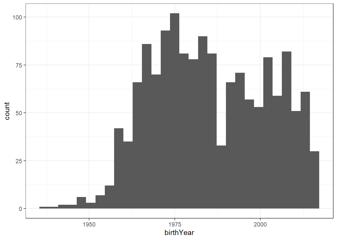
dolphins %>%
  filter(status == "Died") %>%
  mutate(age = statusDate - originDate) %>%
  ggplot(aes(age)) +
  geom_histogram() +
  expand_limits(x = 0) +
  labs(x = "age (days)",
       title = "Dolphin Lifespan")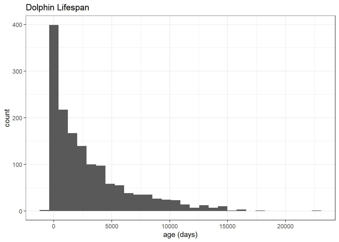
dolphins %>%
  filter(!is.na(birthYear),
         birthYear > 1980) %>%
  count(birthYear, acquisition, sort  = T) %>%
  #complete(birthYear, acquisition, fill = list(n = 0)) %>%
  mutate(
    acquisition = fct_lump(acquisition, n = 5, w = n),
    acquisition = fct_reorder(acquisition, n)
  ) %>%
  group_by(birthYear) %>%
  mutate(percent = n/sum(n)) %>%
  ggplot(aes(birthYear, percent, fill = acquisition)) +
  geom_area() +
  theme_minimal() +
  labs(x = "birth year", y = NULL,
       title = "Birth Year & Acquisition Status",
       subtitle = "Year after 1980") +
  scale_y_continuous(labels = percent)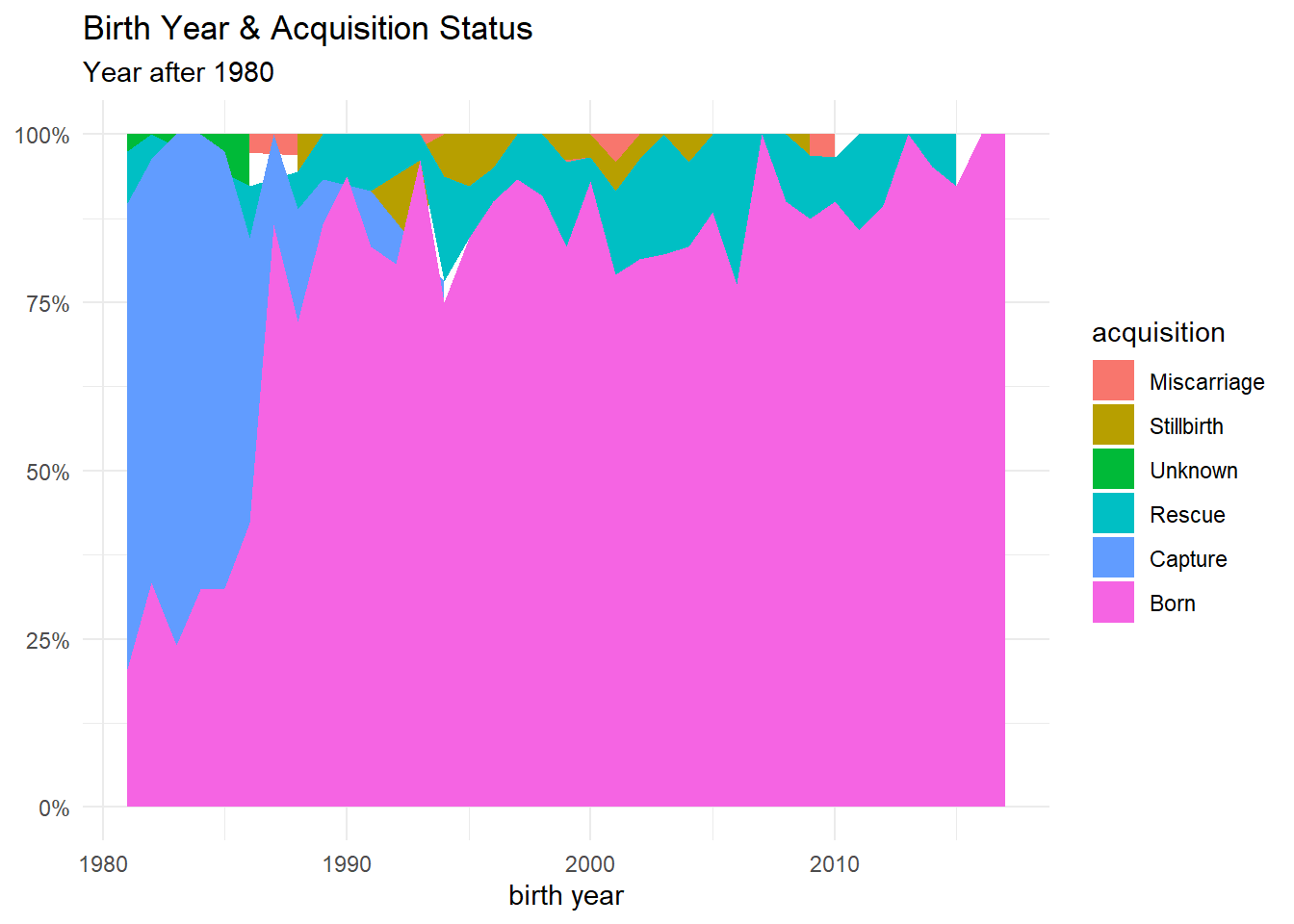
As we can see from the plot above, there is some place where no color covers the plot. Using complete() from dplyr can help us cover the plot perfectly.
dolphins %>%
  filter(!is.na(birthYear),
         birthYear > 1980) %>%
  count(birthYear, acquisition, sort  = T) %>%
  complete(birthYear, acquisition, fill = list(n = 0)) %>%
  mutate(
    acquisition = fct_lump(acquisition, n = 5, w = n),
    acquisition = fct_reorder(acquisition, n)
  ) %>%
  group_by(birthYear) %>%
  mutate(percent = n/sum(n)) %>%
  ggplot(aes(birthYear, percent, fill = acquisition)) +
  geom_area() +
  theme_minimal() +
  labs(x = "birth year", y = NULL,
       title = "Birth Year & Acquisition Status",
       subtitle = "Year after 1980") +
  scale_y_continuous(labels = percent)
The following fuzzyjoin and survival analysis are mostly adopted and inspired by David Robinson’s code for learning purposes. This is my first time using both packages and practicing them here would help me shed some light on how these two packages work, especially for future reference.
fuzzyjoin package
tribble() is a nice and convenient way to compose a tibble.
regexes <- tribble(
  ~ regex, ~ category,
  "Unknown", "Unknown",
  "Gulf of Mexico", "Gulf of Mexico",
  "Florida|FL", "Florida",
  "Texas|TX", "Texas",
  "SeaWorld", "SeaWorld",
  "Pacific", "Pacific Ocean",
  "Atlantic", "Atlantic Ocean"
)
dolphins_annotated <- dolphins %>%
mutate(unique_id = row_number()) %>%
regex_left_join(regexes, c("originLocation" = "regex")) %>%
distinct(unique_id, .keep_all = TRUE) %>%
mutate(category = coalesce(category, originLocation))dolphins_annotated %>%
filter(!is.na(birthYear),
birthYear > 1990) %>%
count(birthYear, originLocation, sort = T) %>%
complete(birthYear, originLocation, fill = list(n = 0)) %>%
mutate(
originLocation = fct_lump(originLocation, n = 5, w = n),
originLocation = fct_reorder(originLocation, n)
) %>%
group_by(birthYear) %>%
mutate(percent = n/sum(n)) %>%
ggplot(aes(birthYear, percent, fill = originLocation)) +
geom_area() +
theme_minimal() +
labs(x = "birth year", y = NULL) +
scale_y_continuous(labels = percent_format())
Survival Analysis
Does sex matter when it comes how long a dolphin can live?
dolphin_sruvival <- dolphins %>%
  filter(status %in% c("Alive", "Died")) %>%
  mutate(deathYear = ifelse(status == "Alive", 2017, year(statusDate)),
         status = ifelse(status == "Alive", 0, 1),
         age = statusDate - originDate
  )%>%
  select(birthYear, deathYear, status, sex, age, acquisition, species)

survival_model1 <- survfit(Surv(age, status) ~ sex, dolphin_sruvival)
tidy(survival_model1) %>%
mutate(
strata = str_remove(strata, "sex=")
) %>%
ggplot(aes(time, estimate, fill = strata, color = strata)) +
geom_line(size = 1) +
geom_ribbon(aes(ymin = conf.low,
ymax = conf.high),
alpha = 0.2) +
scale_y_continuous(labels = percent) +
labs(x = "days", y = "survival percentage")
survival_model2 <- survfit(Surv(birthYear, deathYear, status) ~ sex, dolphin_sruvival %>% filter(deathYear > birthYear))


tidy(survival_model2) %>%
  mutate(
    strata = str_remove(strata, "sex=")
  ) %>%
  ggplot(aes(time, estimate, fill = strata, color = strata)) +
  geom_line(size = 1) +
  geom_ribbon(aes(ymin = conf.low,
              ymax = conf.high),
              alpha = 0.2) +
  scale_y_continuous(labels = percent) +
  labs(x = "years", y = "survival percentage")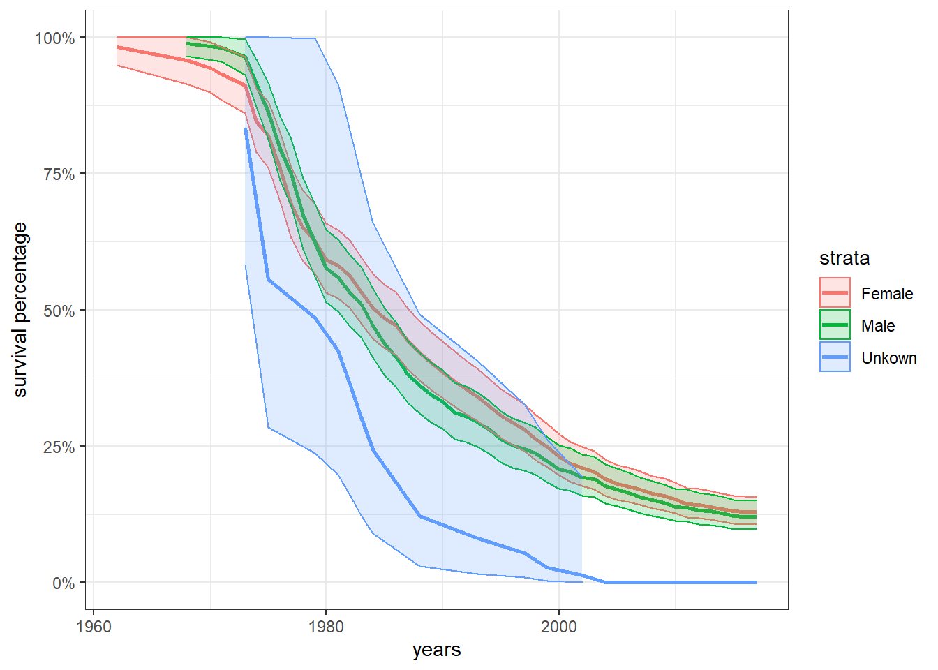
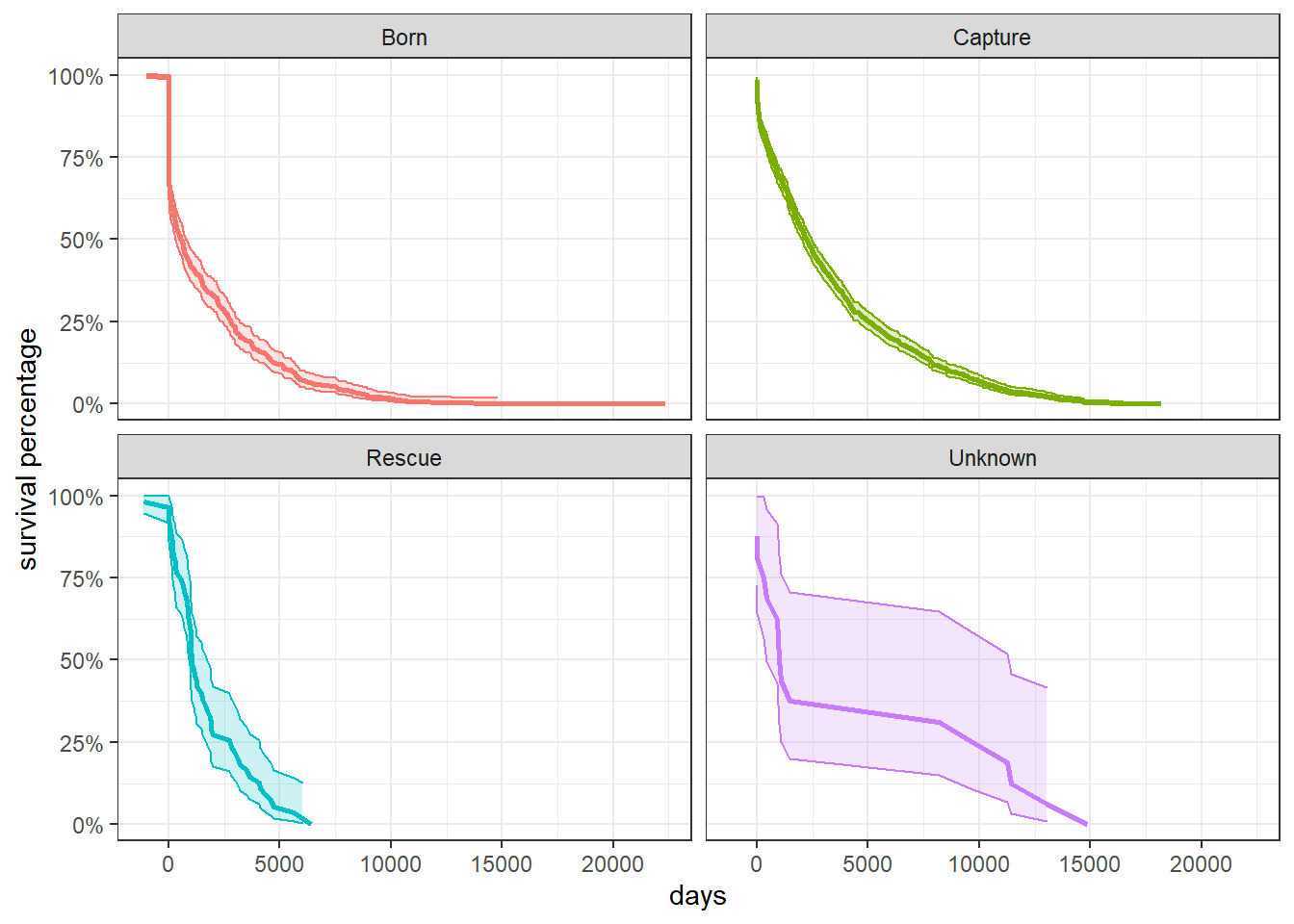
Does acquisition matter when it comes how long a dolphin can live?
survival_model3 <- survfit(Surv(age, status) ~ acquisition, dolphin_sruvival)

tidy(survival_model3) %>%
  mutate(
    strata = str_remove(strata, "acquisition=")
  ) %>%
  ggplot(aes(time, estimate, fill = strata, color = strata)) +
  geom_line(size = 1) +
  geom_ribbon(aes(ymin = conf.low,
              ymax = conf.high),
              alpha = 0.2) +
  scale_y_continuous(labels = percent) +
  labs(x = "days", y = "survival percentage") +
  facet_wrap(~strata) +
  theme(
    legend.position = "none"
  )