Tweet Corpus Text Analysis
The datasets analyzed in this blog post is from TidyTuesday about tweets with hashtag #rstats and #TidyTuesday.
library(tidyverse)
library(tidytext)
library(scales)
library(hms)
library(lubridate)
library(rvest)
library(ggrepel)
theme_set(theme_light())
tt<- read_rds(url("https://github.com/rfordatascience/tidytuesday/blob/master/data/2019/2019-01-01/tidytuesday_tweets.rds?raw=true")) %>%
mutate(time = as_hms(created_at),
date = date(created_at),
account_age = interval(account_created_at, created_at)/ years(1),
week = floor_date(date, "week", week_start = 1)) This is my first time loading a dataset by using read_rds. If the source is a URL, don’t forget to include url().
Checking if user_id and screen_name are one-to-one mapping.
tt %>%
  select(user_id, screen_name) %>%
  distinct() %>%
  count(user_id, screen_name, sort = T)
## # A tibble: 478 x 3
## user_id screen_name n
## <chr> <chr> <int>
## 1 1000252830 xenggg 1
## 2 1001511262545592320 WeAreRLadies 1
## 3 1004392971419123713 marinecdf 1
## 4 1004465754253742082 greens_wgc 1
## 5 1006621907737808896 OliXcl 1
## 6 1009356826801004544 Christi58451746 1
## 7 1010160326137057280 AllieSherier 1
## 8 1012444081 lponnala 1
## 9 1012925456717352960 bidulomique 1
## 10 1016121144 FerreMtrCrtx 1
## # ... with 468 more rowsBased on the output above, it is confirmed that they are one-to-one mapping, which means that no user changed the screen name in the time interval set by the dataset. That is to say, we can use either user_id or screen_name in our further analysis, and using both of them might be repetitious.
Tweets from different platforms
tt %>%
  count(date, source, sort = T) %>%
  mutate(source = fct_lump(source, n = 5, w = n),
         source = fct_reorder(source, n)) %>%
  ggplot(aes(date, n, color = source)) +
  geom_line(size = 1) +
  scale_x_date(date_labels = "%y %b") +
  facet_wrap(~source) +
  theme(
    legend.position = "none",
    axis.text.x = element_text(angle = 90)
  ) +
  labs(x = NULL, y = "# of tweets",
       title = "Tweets from Various Platforms")
Tweet hours and the relevant metrics
tt %>%
  mutate(hour = hour(time)) %>%
  group_by(hour) %>%
  summarize(`total retweets` = sum(retweet_count),
            `total likes` = sum(favorite_count),
            `total tweets` = n()) %>%
  pivot_longer(-hour, names_to = "rt_or_fav", values_to = "sum_of_hour") %>%
  ggplot(aes(hour, sum_of_hour, color = rt_or_fav)) +
  geom_line(size = 1) +
  labs(color = NULL,
       x = "tweet hour",
       y = "# of likes/retweets",
       title = "Tweet Creation Hour with # of Likes/Retweets") +
  scale_x_continuous(breaks = seq(0, 23))
What is interesting is that for followers below 20000, there is a downward trend between the number of years since twitter account created and the number of followers. I guess the reason is that many accounts do not have active tweets, and therefore do not attract followers.
Twitter account age and followers
tt %>%
  filter(followers_count < 20000) %>%
  ggplot(aes(account_age, followers_count)) +
  geom_point() +
  geom_smooth(method = "lm") +
  labs(x = "years since account created", y = "# of followers",
       title = "The Relationship between Account Age & Follower Count") +
  scale_x_continuous(n.breaks = 7)
## `geom_smooth()` using formula 'y ~ x'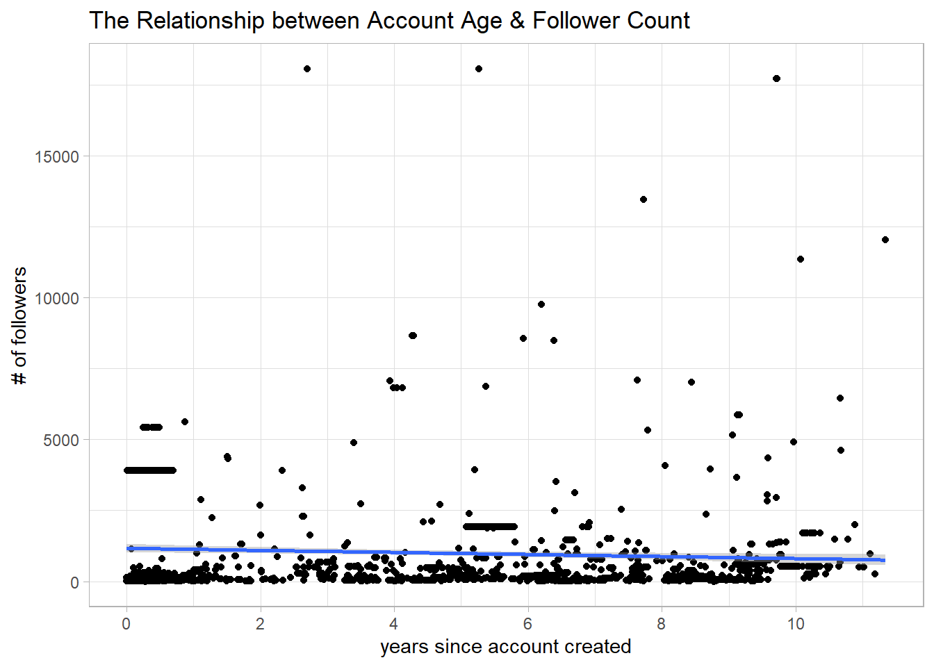
tt %>%
  ggplot(aes(account_age)) +
  geom_histogram()
## `stat_bin()` using `bins = 30`. Pick better value with `binwidth`.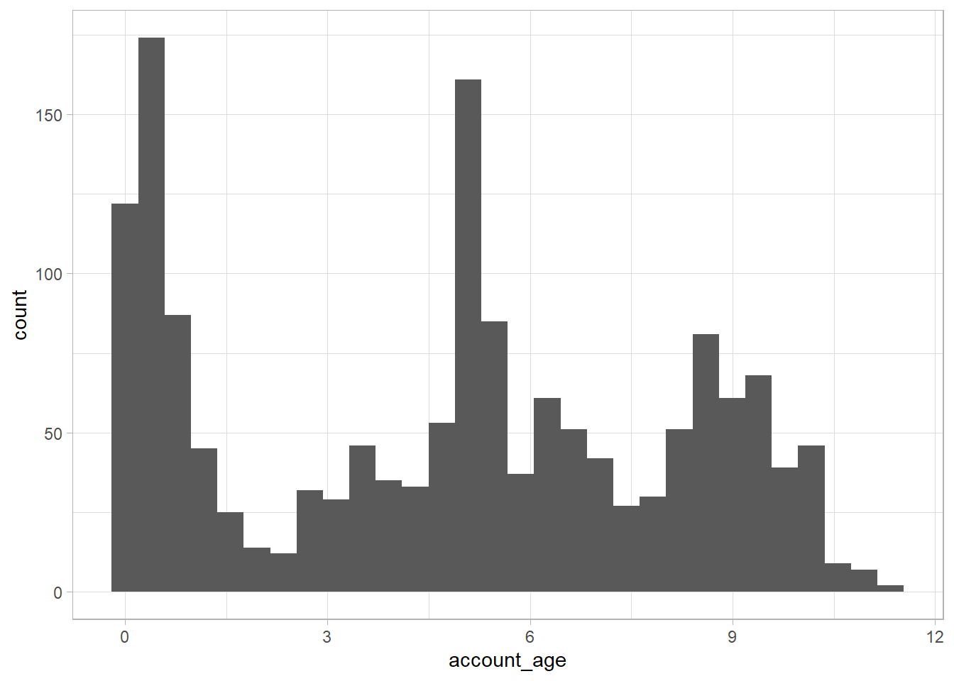
The most popular screen names
tt %>%
  group_by(screen_name) %>%
  summarize(avg_like = mean(favorite_count), avg_retweet = mean(retweet_count)) %>%
  slice_max(avg_like, n = 20) %>%
  mutate(screen_name = fct_reorder(screen_name, avg_like)) %>%
  ggplot(aes(avg_like, screen_name, fill = avg_retweet)) +
  geom_col() +
  labs(x = "average likes",
       y = "twitter name",
       fill = "avg retweets",
       title = "Top 20 Twitter Accounts on Average Likes")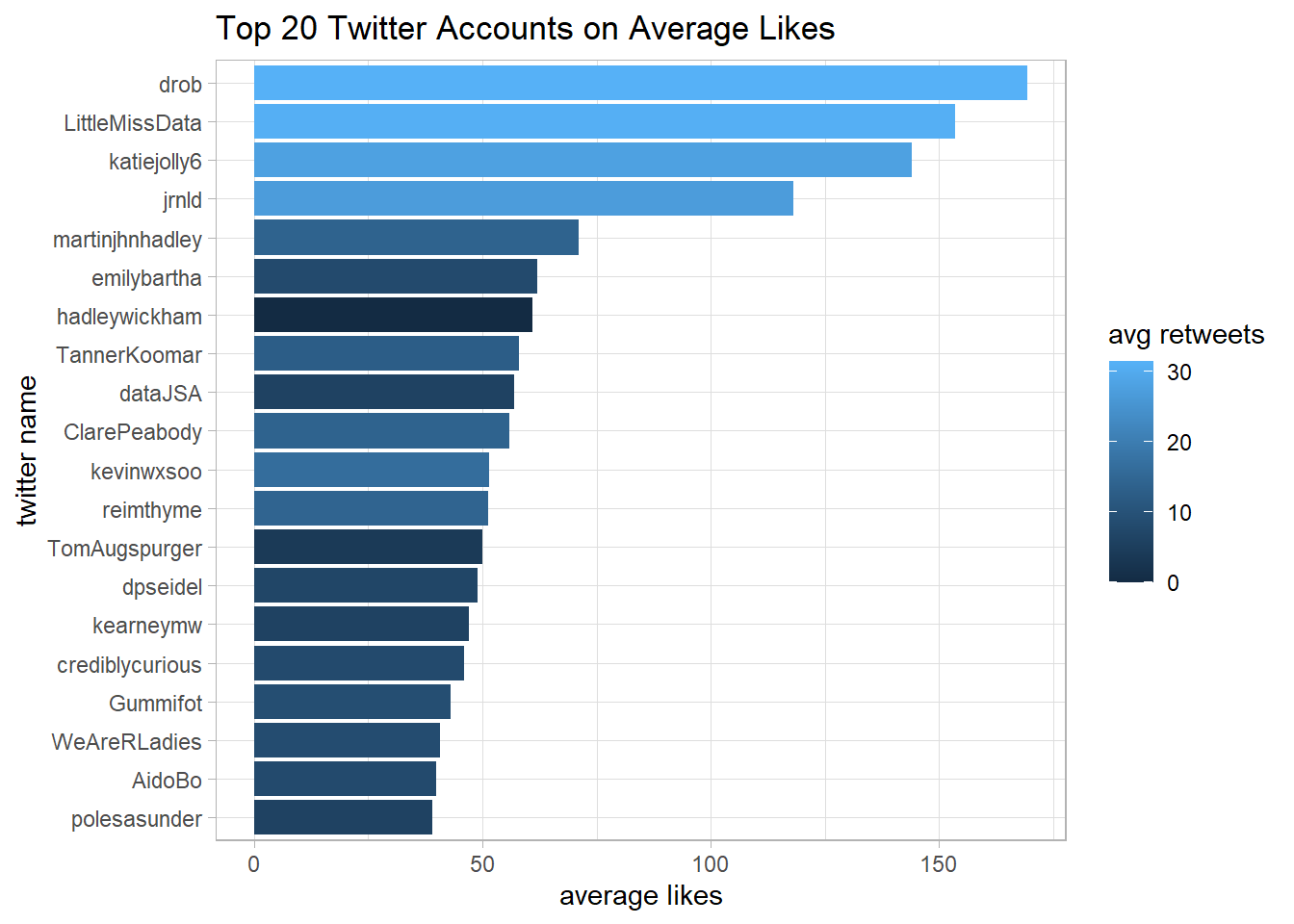
Text analysis
Popular words from tweets
This is my first time knowing that there is a parameter token from unnest_tokens() function, and one of the options for the parameter is tweets. It has made my life much easier to deal with tweet corpus data!
tt %>%
  select(text) %>%
  unnest_tokens(word, text, token = "tweets") %>%
  anti_join(stop_words) %>%
  count(word, sort = T) %>%
  head(20) %>%
  mutate(word = fct_reorder(word, n)) %>%
  ggplot(aes(n, word)) +
  geom_col() +
  labs(x = "# of tweet word frequency",
       y = NULL,
       title = "Top 20 Popular Words from TidyTuesday Tweet Corpus",
       subtitle = "Stop words are removed")
## Using `to_lower = TRUE` with `token = 'tweets'` may not preserve URLs.## Joining, by = "word"
Popular words from twitter account description
tt %>%
  select(description) %>%
  unnest_tokens(word, description, token = "tweets") %>%
  anti_join(stop_words) %>%
  count(word, sort = T) %>%
  head(20) %>%
  mutate(word = fct_reorder(word, n)) %>%
  ggplot(aes(n, word)) +
  geom_col() +
  labs(x = "# of twitter description word frequency",
       y = NULL,
       title = "Top 20 Popular Words from Twitter Description",
       subtitle = "Stop words are removed")
## Using `to_lower = TRUE` with `token = 'tweets'` may not preserve URLs.## Joining, by = "word"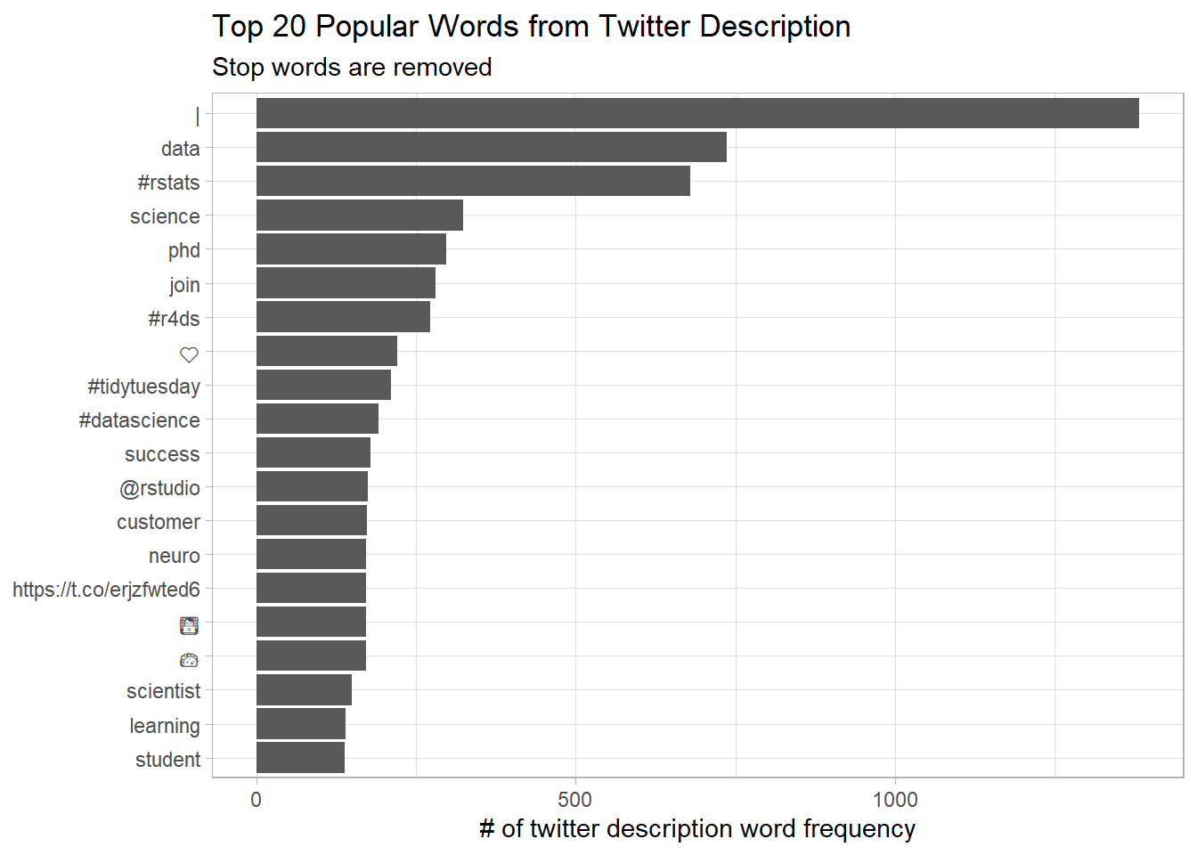
The most popular hashtags
tt %>%
  count(hashtags, sort = T) %>%
  unnest(hashtags) %>%
  group_by(hashtags) %>%
  summarize(total = sum(n)) %>%
  arrange(desc(total)) %>%
  filter(!is.na(hashtags)) %>%
  mutate(
    hashtags = fct_lump(hashtags, n = 20, w = total),
    hashtags = fct_reorder(hashtags, total)
  ) %>%
  ggplot(aes(total, hashtags)) +
  geom_col() +
  labs(x = "# of hashtags", y = "hashtags",
       title = "The 20 Most Popular Hashtags")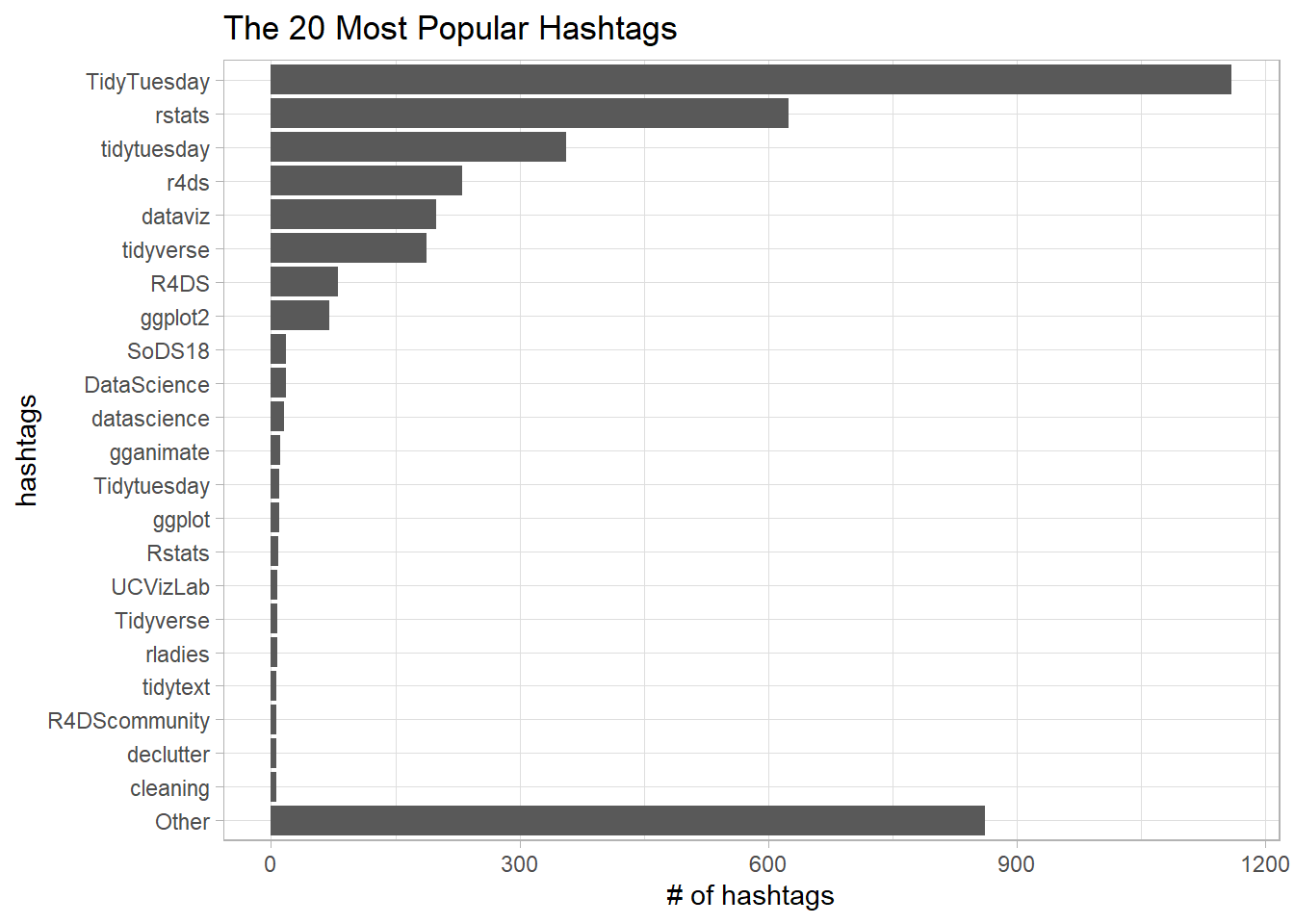
rstats <- read_rds(url("https://github.com/rfordatascience/tidytuesday/blob/master/data/2019/2019-01-01/rstats_tweets.rds?raw=true"))

rstats
## # A tibble: 429,513 x 88
## user_id status_id created_at screen_name text source
## <chr> <chr> <dttm> <chr> <chr> <chr>
## 1 5685812 1075471526902857733 2018-12-19 19:22:47 hrbrmstr "JSON rea~ Buffer
## 2 5685812 994924703063199744 2018-05-11 12:58:28 hrbrmstr "#rstats ~ Twitt~
## 3 5685812 999083117561315329 2018-05-23 00:22:31 hrbrmstr "Whoa. Ju~ Twitt~
## 4 5685812 1064499403073994754 2018-11-19 12:43:29 hrbrmstr "Super gl~ Buffer
## 5 5685812 1003767187088306177 2018-06-04 22:35:21 hrbrmstr "macOS #r~ Twitt~
## 6 5685812 1001808827614990337 2018-05-30 12:53:31 hrbrmstr "Work wit~ Twitt~
## 7 5685812 997045224332496896 2018-05-17 09:24:40 hrbrmstr "Despite ~ Twitt~
## 8 5685812 1001521831889825792 2018-05-29 17:53:06 hrbrmstr "If you n~ Twitt~
## 9 5685812 992214208904343557 2018-05-04 01:27:56 hrbrmstr "A 620 MB~ Twitt~
## 10 5685812 994333160275173376 2018-05-09 21:47:53 hrbrmstr "Hey #rst~ Twitt~
## # ... with 429,503 more rows, and 82 more variables: display_text_width <dbl>,
## # reply_to_status_id <chr>, reply_to_user_id <chr>,
## # reply_to_screen_name <chr>, is_quote <lgl>, is_retweet <lgl>,
## # favorite_count <int>, retweet_count <int>, hashtags <list>, symbols <list>,
## # urls_url <list>, urls_t.co <list>, urls_expanded_url <list>,
## # media_url <list>, media_t.co <list>, media_expanded_url <list>,
## # media_type <list>, ext_media_url <list>, ext_media_t.co <list>, ...There are 639 tweets that are the same from both datasets.
rstats %>%
  inner_join(tt, by = c("user_id", "created_at")) %>%
  dim()
## [1] 639 178Others
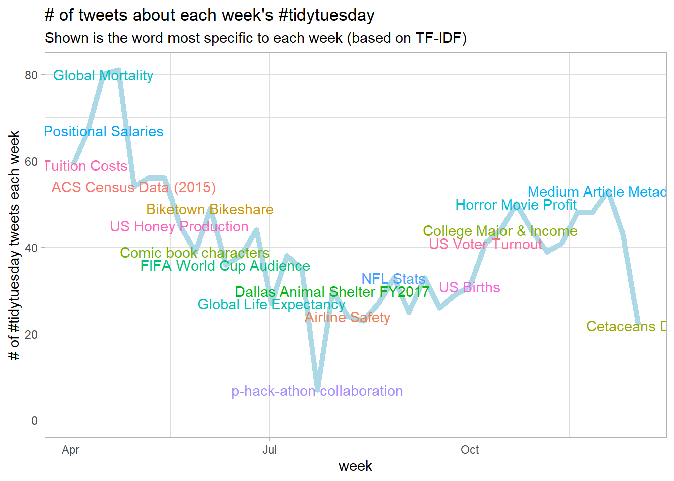
The following code is inspired and largely adopted from David Robinson’s code.
tweet_words <- tt %>%
  select(screen_name, text, retweet_count, favorite_count, created_at, status_id,
         week) %>%
  unnest_tokens(word, text, token = "tweets") %>%
  anti_join(stop_words, by = "word")


word_summary <- tweet_words %>%
  #filter(!screen_name %in% c("thomas_mock", "R4DScommunity")) %>%
  group_by(word) %>%
  summarize(n = n(),
            avg_retweets = exp(mean(log(retweet_count + 1))) - 1,
            avg_favorites = exp(mean(log(favorite_count + 1))) - 1) %>%
  filter(n >= 35) %>%
  arrange(desc(avg_retweets))

week_summary <- tt %>%
  group_by(week) %>%
  summarize(tweets = n(),
            avg_retweets = exp(mean(log(retweet_count + 1))) - 1)

top_words <- tweet_words %>%
  count(word, week) %>%
  bind_tf_idf(word, week, n) %>%
  arrange(desc(tf_idf)) %>%
  distinct(week, .keep_all = TRUE) %>%
  arrange(week)
Grabbing the titles from the TidyTuesday Github page. Why typing ?html_node on RStudio console, the documentation informs me that html_node() has been emerged into html_element().
week_titles <- read_html("https://github.com/rfordatascience/tidytuesday/tree/master/data/2018") %>%
  #html_node(".entry-content") %>%
  html_element("table") %>%
  html_table() %>%
  #tbl_df() %>%
  transmute(week = floor_date(as.Date(Date), "week", week_start = 1),
            title = Data)
week_summary %>%
inner_join(top_words, by = "week") %>%
inner_join(week_titles, by = "week") %>%
ggplot(aes(week, tweets)) +
geom_line(color = "lightblue", size = 2) +
geom_text(aes(label = title, color = title), check_overlap = TRUE) +
expand_limits(y = 0) +
labs(x = "week",
y = "# of #tidytuesday tweets each week",
title = "# of tweets about each week's #tidytuesday",
subtitle = "Shown is the word most specific to each week (based on TF-IDF)") +
theme(
legend.position = "none"
)