Space Launch Data Visualization

Data quality check

There is a typo in the dataset from the column launch_date.

launches %>%
  mutate(year = year(launch_date)) %>%
  filter(year == 2918)

## # A tibble: 1 x 12
##   tag            JD launch_date launch_year type  variant mission agency state_code
##   <chr>       <dbl> <date>            <dbl> <chr> <chr>   <chr>   <chr>  <chr>     
## 1 2018-F01 2787121. 2918-10-11         2018 Soyu~ <NA>    Soyuz ~ RU     RU        
## # ... with 3 more variables: category <chr>, agency_type <chr>, year <dbl>

launch_date is 2918-10-11 but launch_year is 2018. There is a false data entry here.

Time series data visualization

state_text <- launches %>%
  group_by(launch_year, state_code) %>%
  summarize(n = n()) %>%
  filter(n > 10) %>%
  ungroup() %>%
  group_by(state_code) %>%
  slice_max(n, n = 1) %>%
  ungroup() %>%
  distinct(state_code, n, .keep_all = TRUE)

p1 <- launches %>%
  count(launch_year, state_code, sort = T) %>%
  filter(n > 10) %>%
  mutate(state_code = fct_reorder(state_code, n)) %>%
  ggplot(aes(launch_year, n, color = state_code)) +
  geom_line(size = 1) +
  geom_text(data = state_text, aes(label = state_code), check_overlap = T,
            nudge_x = 1, nudge_y = 1,
            vjust = 1,
            size = 3) +
  theme(
    legend.position = "none"
  ) +
  labs(x = "launch year",
       y = "# of launches",
       title = "Yearly # of Rocket Launches > than 10") +
  expand_limits(y = 0) +
  scale_x_continuous(breaks = seq(1960, 2020, by = 5))


p2 <- launches %>%
  count(launch_year, agency_type, sort = T) %>%
  ggplot(aes(launch_year, n, color = agency_type)) +
  geom_line(size = 1) +
  labs(x = "launch year",
       y = "# of launches",
       title = "# of Total Launches") +
  scale_x_continuous(breaks = seq(1960, 2020, by = 5)) +
  scale_y_continuous(breaks = seq(0, 150, 10))

p1 / p2

state_yearly_launches <- launches %>%
  group_by(launch_year, state_code) %>%
  summarize(n = n()) %>%
  left_join(launches %>%
              count(launch_year, sort = T, name = "total_launches"), by = "launch_year") %>%
  mutate(state_ratio = n/total_launches) %>%
  ungroup()

  
state_yearly_launches %>%
  filter(state_code %in% state_text$state_code) %>%
  mutate(state_code = fct_reorder(state_code, -state_ratio, sum)) %>%
  ggplot(aes(launch_year, state_ratio, color = state_code)) +
  geom_line(size = 1) +
  scale_x_continuous(breaks = seq(1960, 2020, by = 5)) +
  scale_y_continuous(labels = percent) +
  labs(x = "launch year",
       y = "yearly state percentage of rocket launches",
       title = "Yearly State Rocket Launch Percentage")

Top types of rockets launched

launches %>%
  count(type, state_code, sort = T) %>%
  mutate(type = fct_lump(type, n = 20, w = n),
         type = fct_reorder(type, n)) %>% 
  filter(type != "Other") %>%
  ggplot(aes(n, type, fill = state_code, label = state_code, group = state_code)) +
  geom_col() +
  geom_text(check_overlap = T, position = position_stack(vjust = 0.5)) +
  theme(
    legend.position = "none",
    axis.title = element_text(size = 13),
    axis.text = element_text(size = 12),
    plot.title = element_text(size = 17)
  ) +
  labs(x = "# of launches",
       y = NULL,
       title = "Top 20 Types of Rockets Launched")

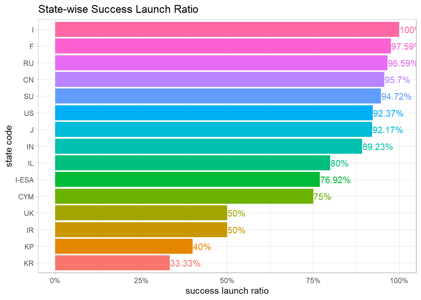
Launch Success or Failure

launches %>%
  count(category, state_code, sort = T) %>%
  group_by(state_code) %>%
  mutate(total_state_launch = sum(n)) %>%
  ungroup() %>%
  mutate(success_ratio = n/total_state_launch) %>%
  filter(category == "success") %>%
  select(-category) %>%
  mutate(state_code = fct_reorder(state_code, success_ratio)) %>%
  ggplot(aes(success_ratio, state_code, fill = state_code)) +
  geom_col() +
  geom_text(aes(label = paste0(round(success_ratio * 100, 2), "%"),
                color = state_code), hjust = -0.01) +
  scale_x_continuous(labels = percent, breaks = seq(0,1, 0.25))  +
  labs(x = "success launch ratio",
       y = "state code",
       title = "State-wise Success Launch Ratio") +
  theme(
    legend.position = "none"
  )

State-wise agency type

agencies %>%
  group_by(state_code, agency_type) %>%
  summarize(count = n()) %>%
  ungroup() %>%
  group_by(state_code) %>%
  mutate(total_state_count = sum(count),
         agency_type = factor(agency_type, c("state", "private", "startup"))) %>%
  ungroup() %>%
  mutate(type_ratio = count/total_state_count,
         state_code = reorder_within(state_code, type_ratio, agency_type)) %>%
  ggplot(aes(type_ratio, state_code, fill = state_code)) +
  geom_col() +
  facet_wrap(~agency_type, scales = "free_y")  +
  scale_x_continuous(labels = percent) +
  scale_y_reordered() +
  theme(
    legend.position = "none",
    strip.text = element_text(size = 15, face = "bold")
  ) +
  labs(x = "percentage of state-wise agency type",
       y = "state code",
       title = "State-wise Agency Type Percentage",
       subtitle = "Percentage is computed by grouping by each cournty")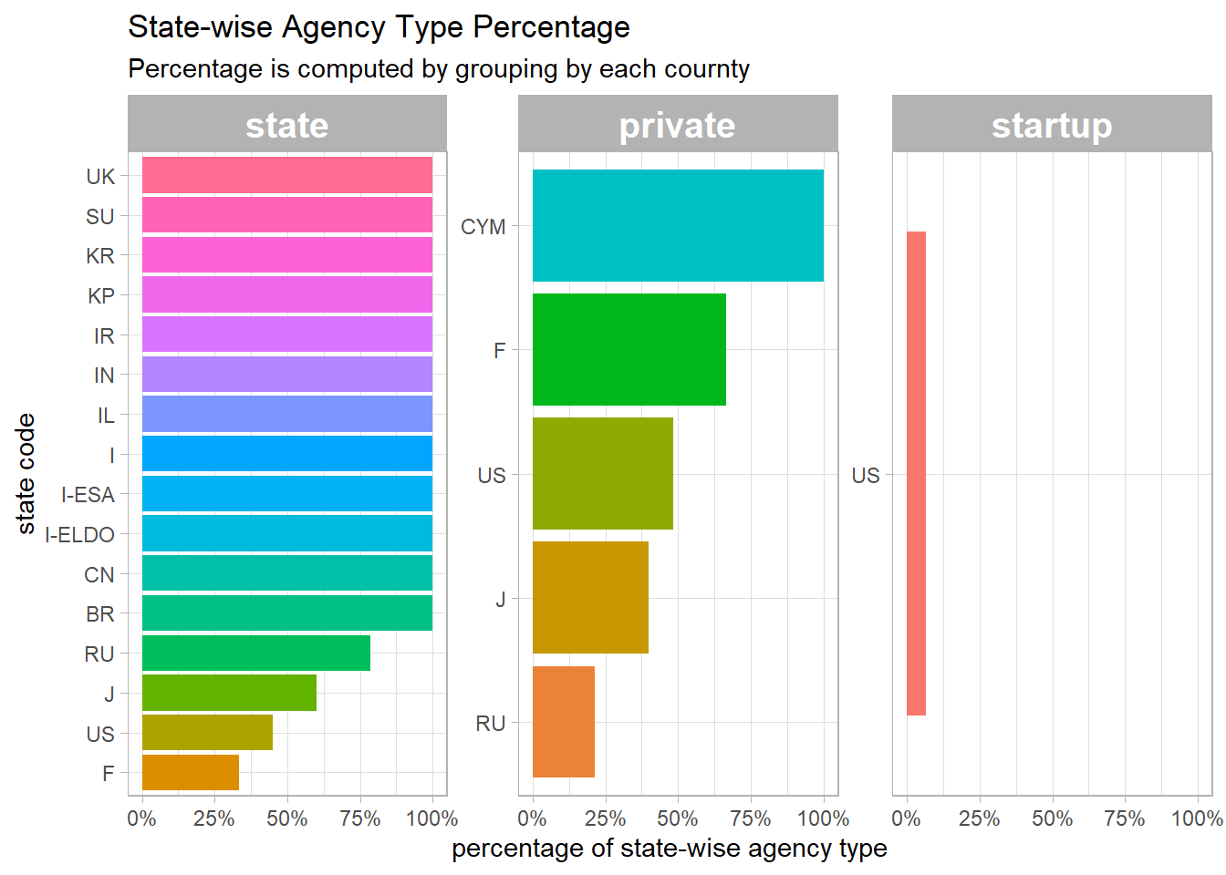

Learning resources

The following code/idea is referenced/inspired by David Robinson (here is his code).

Now focus on private + startup launches

private_startup_launches <- launches %>%
  filter(agency_type %in% c("startup", "private")) %>%
  inner_join(agencies %>%
              select(agency, agency_name = name, short_name), by = "agency") %>%
  mutate(agency_name_lumped = fct_lump(agency_name, 6),
         agency_name_lumped = if_else(agency_name_lumped == "Other" & state_code == "US",
                                     "Other US", as.character(agency_name_lumped)))


private_startup_launches %>%
  count(agency_name_lumped, state_code, sort = TRUE) %>%
  mutate(agency_name_lumped = fct_reorder(agency_name_lumped, n, sum)) %>%
  ggplot(aes(agency_name_lumped, n, fill = state_code)) +
  geom_col() +
  coord_flip() +
  labs(x = "",
       y = "# of launches overall",
       title = "What private/startup agencies have had the most launches?",
       fill = "Country")

Launch per vehicle type

vehicles <- launches %>%
  filter(year(launch_date) < 2020) %>%
  group_by(type, state_code) %>%
  summarize(first_launch = min(launch_date),
            last_launch = max(launch_date),
            num_of_launches = n()) %>%
  ungroup()

## `summarise()` has grouped output by 'type'. You can override using the `.groups` argument.

The functions getting vehicle types for a specific country in different time intervals

country_vehicles <- function(country1, country2 = "", mid_point = 300, country_name_for_title, num_of_filter = 0){
  vehicles %>% 
  filter(state_code == country1 | state_code == country2,
         year(first_launch) < year(last_launch)) %>%
  mutate(type = fct_reorder(type, first_launch, min)) %>%
  filter(num_of_launches > num_of_filter) %>%
  ggplot(aes(first_launch, type, color = num_of_launches, size = num_of_launches)) +
  geom_point() +
  geom_errorbar(aes(xmin = first_launch, xmax = last_launch), size = 1) +
  scale_x_date(date_breaks = "5 years", date_labels = "%Y") +
  scale_color_gradient2(low = "blue",
                        high = "red",
                        midpoint = mid_point) +
  labs(x = "launching time interval",
       y = "vehicle type",
       title = paste(country_name_for_title, "Rocket Types in Different Time Intervals"),
       color = "# of launches",
       size = "# of launches") 
  
}

Russian Vehicles

country_vehicles(country1 = "SU",country2 = "RU", country_name_for_title = "Soviet Union/Russian")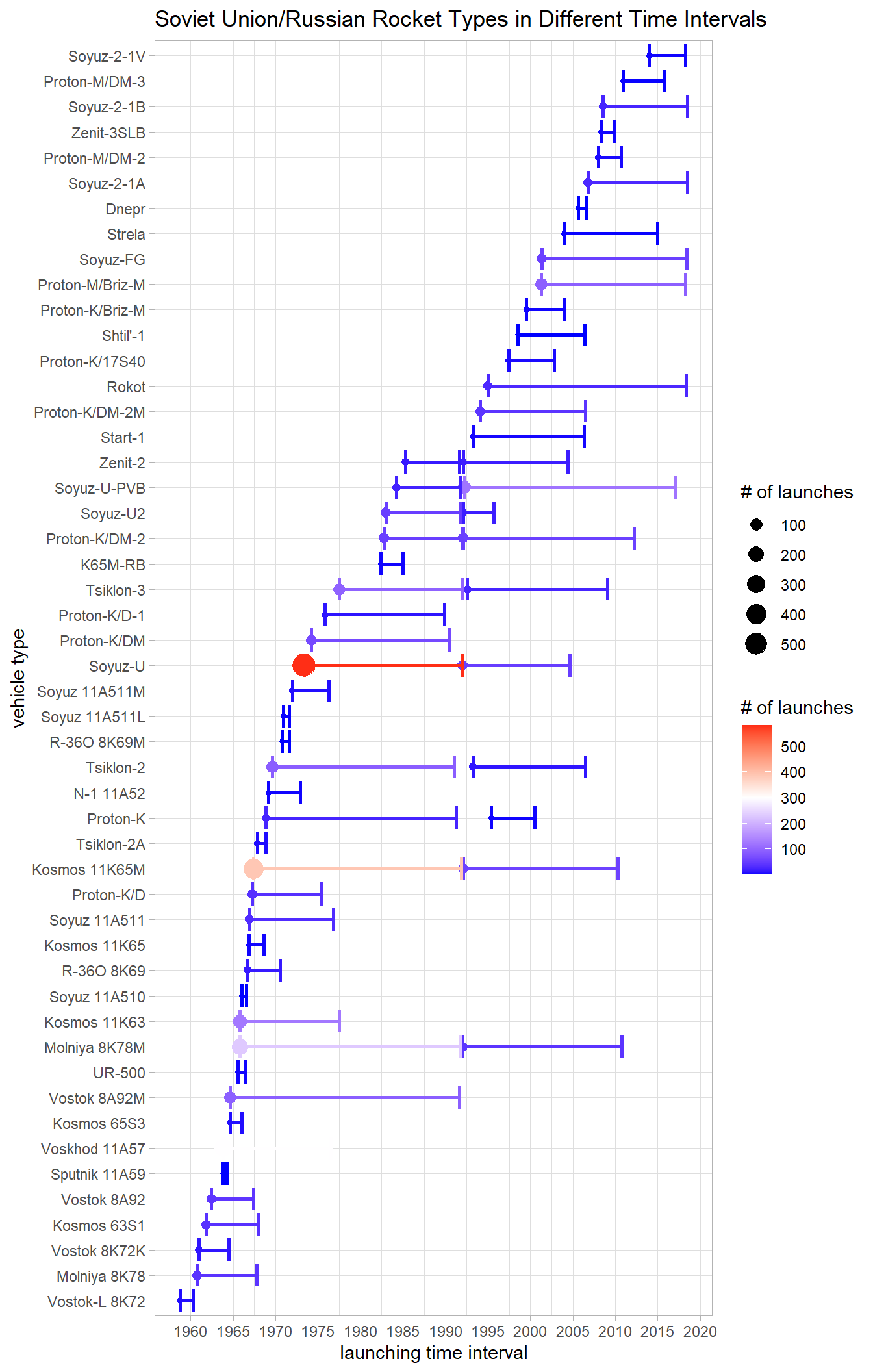 

US Vehicles

country_vehicles(country1 = "US", country_name_for_title = "US", mid_point = 50, num_of_filter = 10) 

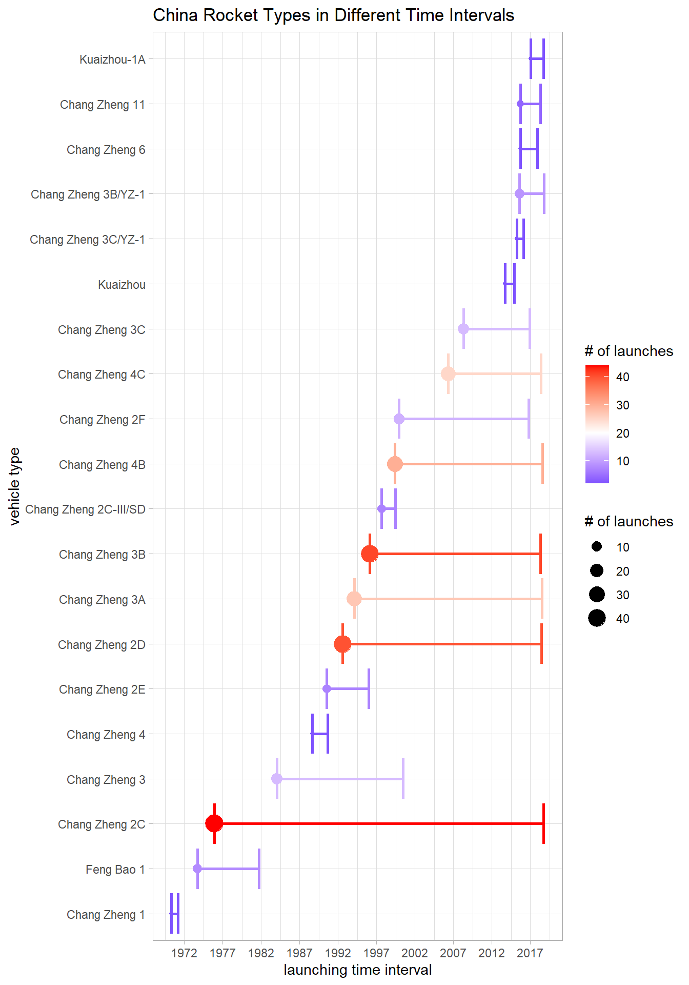
Chinese Vehicles

country_vehicles(country1 = "CN", country_name_for_title = "China", mid_point = 20)