Analyzing US Dairy Consumption with Time Series Prediction (sweep package used)
Thu, Sep 30, 2021
7-minute read
The 5 dairy-related datasets in this blog post we analyze are from TidyTuesday.
library(tidyverse)
library(lubridate)
library(sweep)
library(timetk)
library(forecast)
milk_products_facts <- read_csv("https://raw.githubusercontent.com/rfordatascience/tidytuesday/master/data/2019/2019-01-29/milk_products_facts.csv")
cheese <- read_csv("https://raw.githubusercontent.com/rfordatascience/tidytuesday/master/data/2019/2019-01-29/clean_cheese.csv")
milk_sales <- read_csv("https://raw.githubusercontent.com/rfordatascience/tidytuesday/master/data/2019/2019-01-29/fluid_milk_sales.csv")
cows <- read_csv("https://raw.githubusercontent.com/rfordatascience/tidytuesday/master/data/2019/2019-01-29/milkcow_facts.csv")
state_milk <- read_csv("https://raw.githubusercontent.com/rfordatascience/tidytuesday/master/data/2019/2019-01-29/state_milk_production.csv")Check data quality
skimr::skim(milk_products_facts)| Name | milk_products_facts |
| Number of rows | 43 |
| Number of columns | 18 |
| _______________________ | |
| Column type frequency: | |
| numeric | 18 |
| ________________________ | |
| Group variables | None |
Variable type: numeric
| skim_variable | n_missing | complete_rate | mean | sd | p0 | p25 | p50 | p75 | p100 | hist |
|---|---|---|---|---|---|---|---|---|---|---|
| year | 0 | 1 | 1996.00 | 12.56 | 1975.00 | 1985.50 | 1996.00 | 2006.50 | 2017.00 | ▇▇▇▇▇ |
| fluid_milk | 0 | 1 | 202.91 | 27.03 | 149.00 | 183.00 | 205.00 | 223.50 | 247.00 | ▃▆▆▇▅ |
| fluid_yogurt | 0 | 1 | 7.16 | 4.34 | 1.97 | 3.78 | 5.87 | 11.31 | 14.93 | ▇▅▂▂▅ |
| butter | 0 | 1 | 4.71 | 0.43 | 4.19 | 4.37 | 4.54 | 4.91 | 5.69 | ▇▅▃▁▂ |
| cheese_american | 0 | 1 | 11.95 | 1.50 | 8.15 | 11.28 | 12.12 | 12.95 | 15.06 | ▂▂▇▇▂ |
| cheese_other | 0 | 1 | 14.71 | 4.82 | 6.13 | 10.68 | 15.26 | 18.96 | 22.05 | ▆▃▇▅▇ |
| cheese_cottage | 0 | 1 | 3.13 | 0.86 | 2.07 | 2.56 | 2.65 | 4.03 | 4.63 | ▇▇▂▃▅ |
| evap_cnd_canned_whole_milk | 0 | 1 | 2.04 | 0.71 | 0.94 | 1.49 | 1.84 | 2.34 | 3.95 | ▇▇▃▃▁ |
| evap_cnd_bulk_whole_milk | 0 | 1 | 0.81 | 0.29 | 0.44 | 0.58 | 0.70 | 1.06 | 1.46 | ▇▂▃▃▂ |
| evap_cnd_bulk_and_can_skim_milk | 0 | 1 | 4.32 | 0.82 | 3.02 | 3.64 | 4.24 | 5.17 | 5.58 | ▆▆▅▂▇ |
| frozen_ice_cream_regular | 0 | 1 | 15.63 | 1.65 | 12.47 | 14.69 | 15.71 | 17.06 | 18.21 | ▃▃▇▃▆ |
| frozen_ice_cream_reduced_fat | 0 | 1 | 6.40 | 0.43 | 5.67 | 6.08 | 6.33 | 6.61 | 7.55 | ▆▇▇▃▁ |
| frozen_sherbet | 0 | 1 | 1.14 | 0.15 | 0.80 | 1.11 | 1.18 | 1.22 | 1.36 | ▂▁▃▇▂ |
| frozen_other | 0 | 1 | 3.13 | 1.37 | 1.35 | 2.27 | 2.91 | 3.76 | 6.54 | ▆▇▂▁▂ |
| dry_whole_milk | 0 | 1 | 0.31 | 0.14 | 0.09 | 0.20 | 0.30 | 0.40 | 0.60 | ▇▆▅▇▅ |
| dry_nonfat_milk | 0 | 1 | 3.02 | 0.53 | 2.12 | 2.62 | 3.05 | 3.31 | 4.28 | ▅▅▇▂▂ |
| dry_buttermilk | 0 | 1 | 0.23 | 0.05 | 0.17 | 0.20 | 0.20 | 0.25 | 0.39 | ▇▂▁▂▁ |
| dry_whey | 0 | 1 | 3.05 | 0.66 | 1.89 | 2.40 | 3.02 | 3.65 | 4.09 | ▆▆▅▆▇ |
skimr::skim(cheese)| Name | cheese |
| Number of rows | 48 |
| Number of columns | 17 |
| _______________________ | |
| Column type frequency: | |
| numeric | 17 |
| ________________________ | |
| Group variables | None |
Variable type: numeric
| skim_variable | n_missing | complete_rate | mean | sd | p0 | p25 | p50 | p75 | p100 | hist |
|---|---|---|---|---|---|---|---|---|---|---|
| Year | 0 | 1.00 | 1993.50 | 14.00 | 1970.00 | 1981.75 | 1993.50 | 2005.25 | 2017.00 | ▇▇▇▇▇ |
| Cheddar | 0 | 1.00 | 8.89 | 1.52 | 5.79 | 8.30 | 9.52 | 9.92 | 11.07 | ▃▁▁▇▃ |
| American Other | 0 | 1.00 | 2.62 | 0.65 | 1.20 | 2.22 | 2.58 | 2.97 | 3.99 | ▁▅▇▃▃ |
| Mozzarella | 0 | 1.00 | 6.86 | 3.43 | 1.19 | 3.18 | 7.70 | 9.97 | 11.73 | ▇▂▃▆▇ |
| Italian other | 0 | 1.00 | 2.15 | 0.73 | 0.87 | 1.52 | 2.19 | 2.75 | 3.49 | ▅▃▇▃▃ |
| Swiss | 0 | 1.00 | 1.16 | 0.11 | 0.88 | 1.07 | 1.17 | 1.24 | 1.35 | ▁▅▆▇▅ |
| Brick | 0 | 1.00 | 0.05 | 0.03 | 0.01 | 0.03 | 0.05 | 0.07 | 0.12 | ▇▂▅▂▃ |
| Muenster | 0 | 1.00 | 0.34 | 0.09 | 0.17 | 0.28 | 0.34 | 0.40 | 0.53 | ▃▇▆▅▂ |
| Cream and Neufchatel | 0 | 1.00 | 1.74 | 0.69 | 0.61 | 1.10 | 2.05 | 2.35 | 2.64 | ▅▃▂▃▇ |
| Blue | 12 | 0.75 | 0.20 | 0.06 | 0.15 | 0.16 | 0.17 | 0.18 | 0.32 | ▇▁▁▁▂ |
| Other Dairy Cheese | 0 | 1.00 | 1.02 | 0.36 | 0.41 | 0.75 | 0.97 | 1.29 | 1.59 | ▇▇▅▇▇ |
| Processed Cheese | 0 | 1.00 | 4.33 | 0.63 | 3.31 | 3.82 | 4.42 | 4.80 | 5.44 | ▇▇▃▇▅ |
| Foods and spreads | 0 | 1.00 | 3.16 | 0.44 | 1.91 | 2.99 | 3.22 | 3.44 | 3.98 | ▂▁▅▇▃ |
| Total American Chese | 0 | 1.00 | 11.51 | 1.95 | 7.00 | 10.81 | 11.83 | 12.84 | 15.06 | ▂▂▅▇▂ |
| Total Italian Cheese | 0 | 1.00 | 9.01 | 4.15 | 2.05 | 4.68 | 9.95 | 12.73 | 15.21 | ▇▃▅▇▇ |
| Total Natural Cheese | 0 | 1.00 | 25.35 | 7.37 | 11.37 | 19.47 | 26.29 | 31.78 | 37.23 | ▅▅▇▇▇ |
| Total Processed Cheese Products | 0 | 1.00 | 7.49 | 0.87 | 5.53 | 6.90 | 7.59 | 8.20 | 8.75 | ▂▅▆▇▇ |
Milk products facts
milk_pivot <- milk_products_facts %>%
  pivot_longer(-year, names_to = "product", values_to = "consumption")

milk_pivot %>%
  mutate(product = str_replace_all(product, "_", " ")) %>%
  ggplot(aes(year, consumption, color = product)) +
  geom_line(aes(group = 1), size = 2, show.legend = FALSE) +
  facet_wrap(~product, scales = "free_y") +
  expand_limits(y = 0) +
  theme(
    strip.text = element_text(size = 13, face = "bold")
  )  +
  labs(y = "lbs per person",
title = "Milk Product Consumption (lbs per person)") 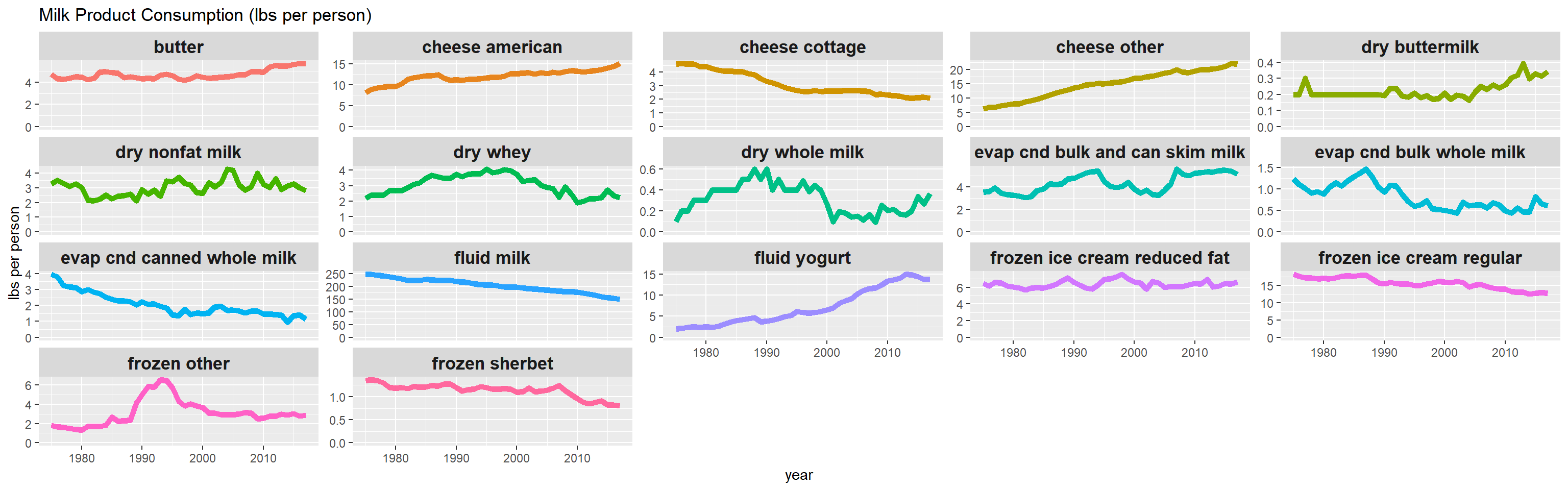
Time series prediction
This section is inspired by David Robinson’s code, and this is also the first time of me using sweep and timetk packages.
milk_productes_tidied <- milk_pivot %>%
  separate(product, c("category", "product"), sep = "_",
           extra = "merge", fill = "right")%>%
  mutate(
    product = coalesce(product, category),
    product = str_to_title(str_replace_all(product, "_", " ")),
    category = str_to_title(category)
  )
milk_ts <- milk_productes_tidied %>%
mutate(year = make_date(year)) %>%
nest(-c(category, product)) %>%
mutate(ts = map(data, tk_ts, start = 1975))
milk_ets <- milk_ts %>%
mutate(model = map(ts, ets))
# the following commented code does not work due to tidyr update
# milk_ets %>%
# unnest(map(model, sw_glance))
# This is the correct way to do it
milk_ets %>%
mutate(glanced = map(model, sw_glance)) %>%
unnest(glanced)## # A tibble: 17 x 17
## category product data ts model model.desc sigma logLik AIC BIC
## <chr> <chr> <list> <lis> <lis> <chr> <dbl> <dbl> <dbl> <dbl>
## 1 Fluid Milk <tibb~ <ts ~ <ets> ETS(A,A,N) 2.05 -110. 229. 238.
## 2 Fluid Yogurt <tibb~ <ts ~ <ets> ETS(M,A,N) 0.0694 -40.3 90.7 99.5
## 3 Butter Butter <tibb~ <ts ~ <ets> ETS(A,N,N) 0.192 -8.92 23.8 29.1
## 4 Cheese American <tibb~ <ts ~ <ets> ETS(A,Ad,~ 0.352 -33.3 78.7 89.3
## 5 Cheese Other <tibb~ <ts ~ <ets> ETS(M,A,N) 0.0214 -26.4 62.7 71.5
## 6 Cheese Cottage <tibb~ <ts ~ <ets> ETS(A,Ad,~ 0.0799 30.5 -48.9 -38.4
## 7 Evap Cnd Can~ <tibb~ <ts ~ <ets> ETS(A,Ad,~ 0.186 -5.91 23.8 34.4
## 8 Evap Cnd Bul~ <tibb~ <ts ~ <ets> ETS(A,N,N) 0.128 8.42 -10.8 -5.56
## 9 Evap Cnd Bul~ <tibb~ <ts ~ <ets> ETS(A,N,N) 0.378 -38.0 81.9 87.2
## 10 Frozen Ice Cre~ <tibb~ <ts ~ <ets> ETS(M,N,N) 0.0286 -45.4 96.7 102.
## 11 Frozen Ice Cre~ <tibb~ <ts ~ <ets> ETS(M,N,N) 0.0586 -37.6 81.1 86.4
## 12 Frozen Sherbet <tibb~ <ts ~ <ets> ETS(A,N,N) 0.0510 48.1 -90.2 -84.9
## 13 Frozen Other <tibb~ <ts ~ <ets> ETS(M,N,N) 0.172 -49.0 104. 109.
## 14 Dry Whole M~ <tibb~ <ts ~ <ets> ETS(A,N,N) 0.0782 29.8 -53.5 -48.2
## 15 Dry Nonfat ~ <tibb~ <ts ~ <ets> ETS(M,N,N) 0.148 -44.9 95.7 101.
## 16 Dry Butterm~ <tibb~ <ts ~ <ets> ETS(M,N,N) 0.141 69.7 -133. -128.
## 17 Dry Whey <tibb~ <ts ~ <ets> ETS(A,N,N) 0.260 -22.0 50.0 55.3
## # ... with 7 more variables: ME <dbl>, RMSE <dbl>, MAE <dbl>, MPE <dbl>,
## # MAPE <dbl>, MASE <dbl>, ACF1 <dbl>milk_ts %>%
crossing(model_name = c("auto.arima", "ets")) %>%
mutate(model = map2(model_name, ts, ~ invoke(.x, list(.y))),
forecast = map(model, forecast, h = 10)) %>%
mutate(sweeped = map(forecast, sw_sweep)) %>%
unnest(sweeped) %>%
ggplot(aes(index, consumption, color = model_name, lty = key)) +
geom_line(size = 1) +
geom_ribbon(aes(ymin = lo.95, ymax = hi.95, fill = model_name), alpha = .5) +
facet_wrap(~ product, scales = "free_y") +
theme(strip.text = element_text(size = 13, face = "bold")) +
expand_limits(y = 0) +
scale_x_continuous(breaks = c(1980, 2000, 2020)) +
scale_linetype_discrete(guide = FALSE) +
labs(x = "Year",
y = "Average US consumption (lbs per person)",
title = "Forecasted consumption of dairy products",
subtitle = "Based on USDA data 1975-2017. Showing 95% prediction intervals.",
color = "Model")
Cheese
cheese %>%
  rename(year = Year) %>%
  pivot_longer(-year, names_to = "product", values_to = "consumption") %>%
  ggplot(aes(year, consumption, color = product)) +
  geom_line(size = 2, show.legend = FALSE) +
  facet_wrap(~product, scales = "free_y") +
  expand_limits(y = 0) +
  theme(
    strip.text = element_text(size = 15, face = "bold")
  )  +
  labs(y = "lbs per person",
title = "Cheese Product Consumption (lbs per person)") 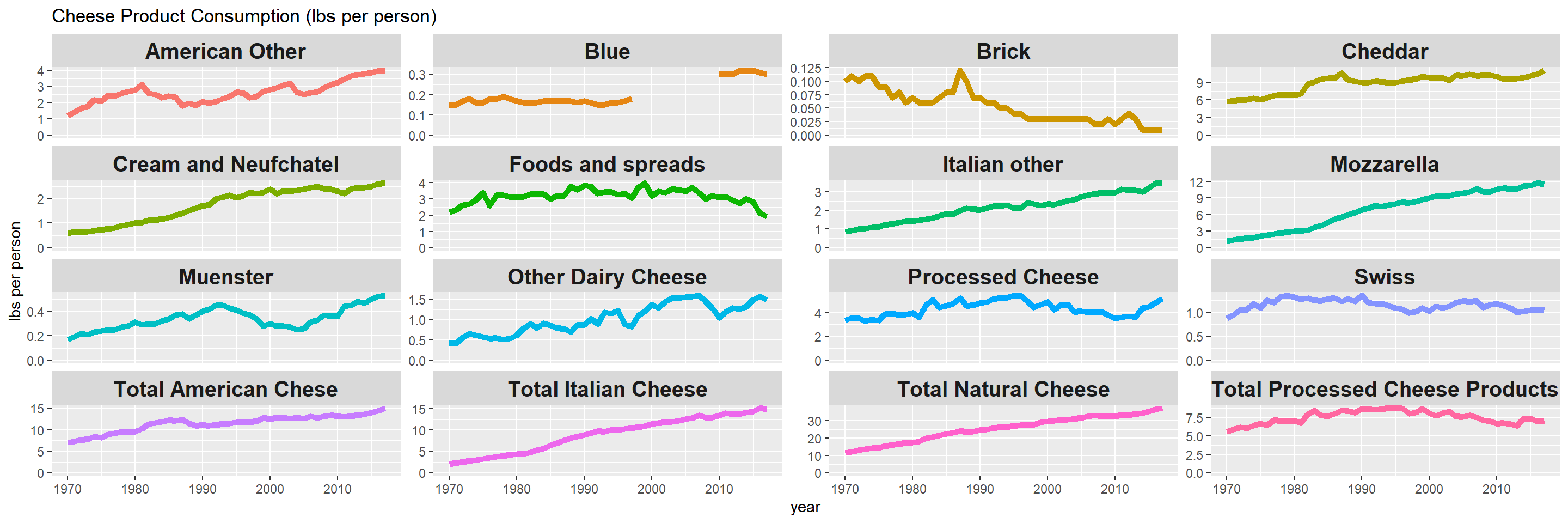
Milk sales
milk_sales %>%
  ggplot(aes(year, pounds, color = milk_type)) +
  geom_line(show.legend = FALSE, size = 2) +
  facet_wrap(~milk_type) +
  expand_limits(y = 0) +
  theme(
    strip.text = element_text(size = 15, face = "bold")
  )  +
labs(title = "Fluid Milk Sales (Pounds)") 
milk_sales %>%
  ggplot(aes(year, pounds, color = milk_type)) +
  geom_line(show.legend = FALSE, size = 2) +
  facet_wrap(~milk_type, scales = "free") +
  expand_limits(y = 0) +
  theme(
    strip.text = element_text(size = 15, face = "bold")
  )  +
labs(title = "Free-scale Fluid Milk Sales (Pounds)") 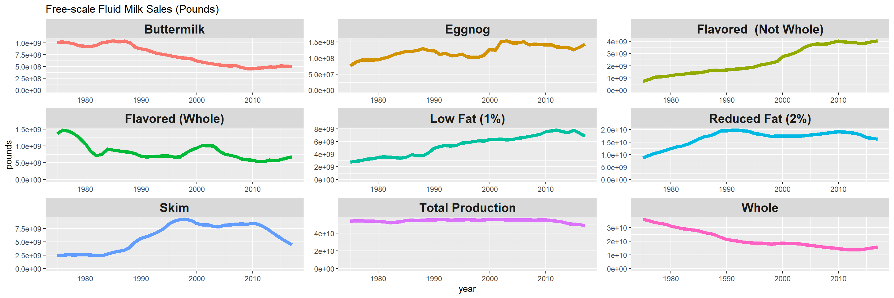
Cows facts
cows %>%
  ggplot(aes(year, milk_per_cow)) +
  geom_line() +
  expand_limits(y = 0)
cows %>%
  ggplot(aes(year, avg_milk_cow_number)) +
  geom_line() +
  expand_limits(y = 0)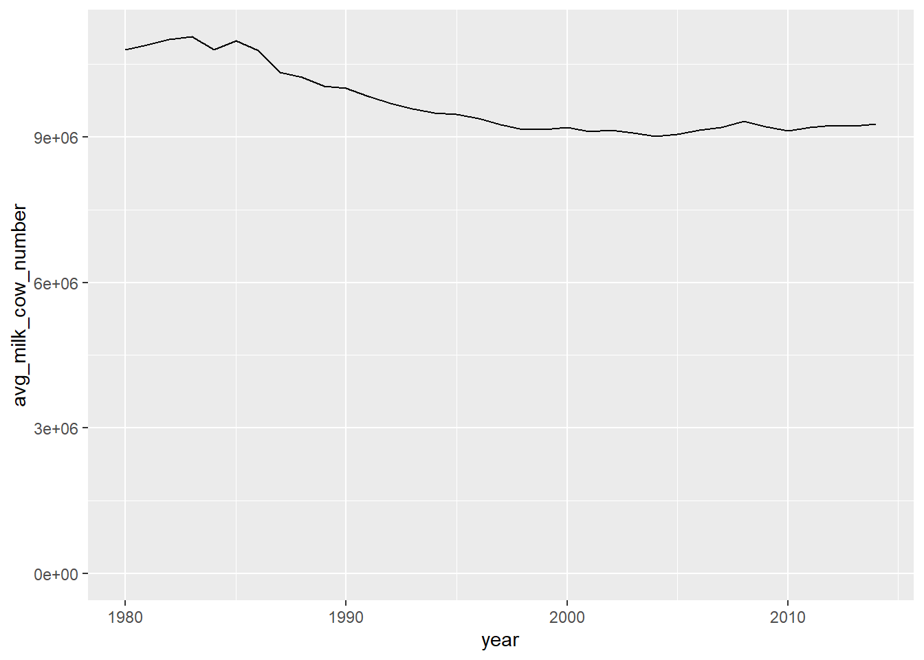
Each cow produced more milk annually from 1980 to 2010, although the # of cows decreased in the same time interval.
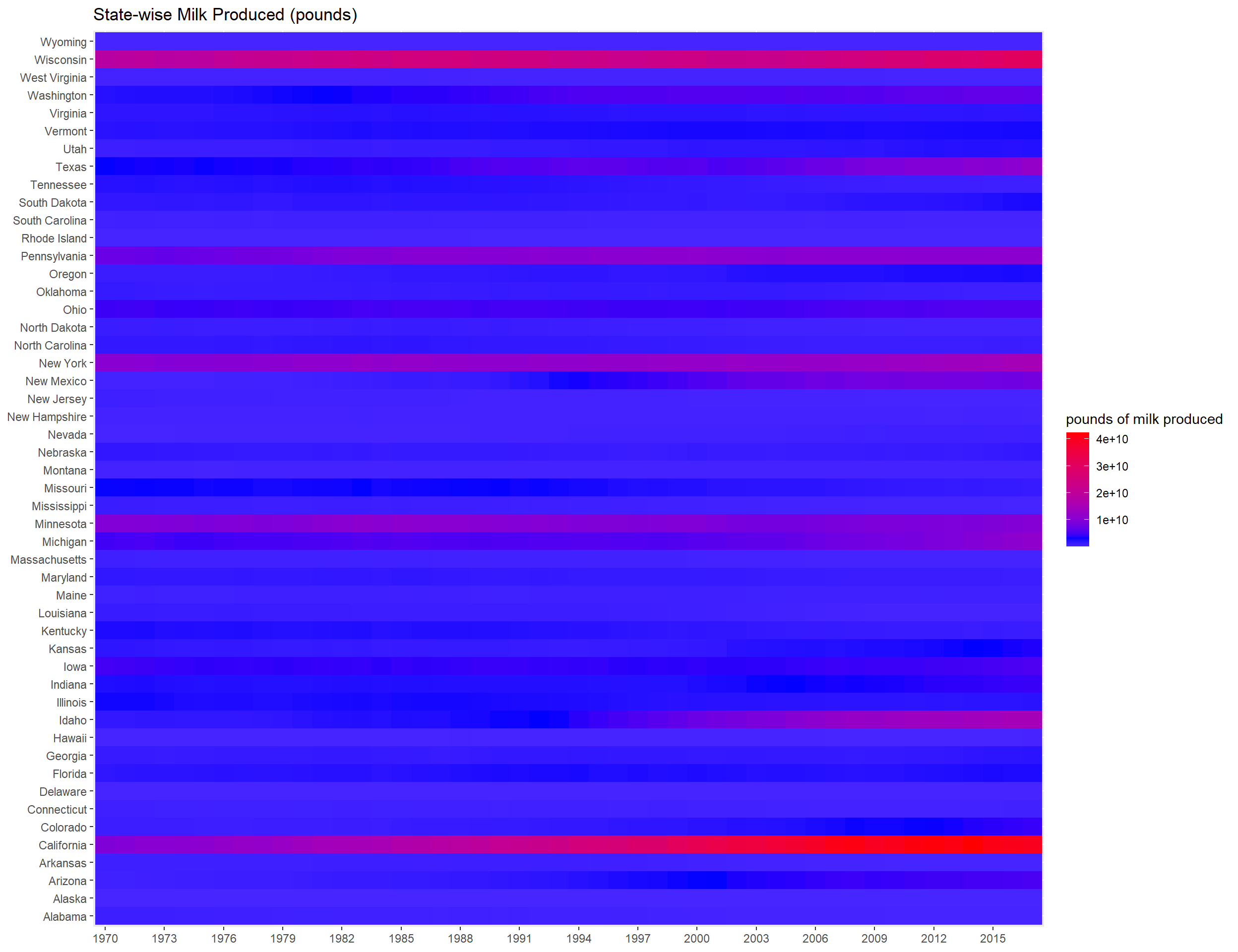
Milk production in each state
state_milk %>%
  ggplot(aes(year, state, size = milk_produced, color = state)) +
  geom_point() +
  scale_color_discrete(guide = FALSE) +
  labs(y = NULL)
## Warning: It is deprecated to specify `guide = FALSE` to remove a guide. Please
## use `guide = "none"` instead.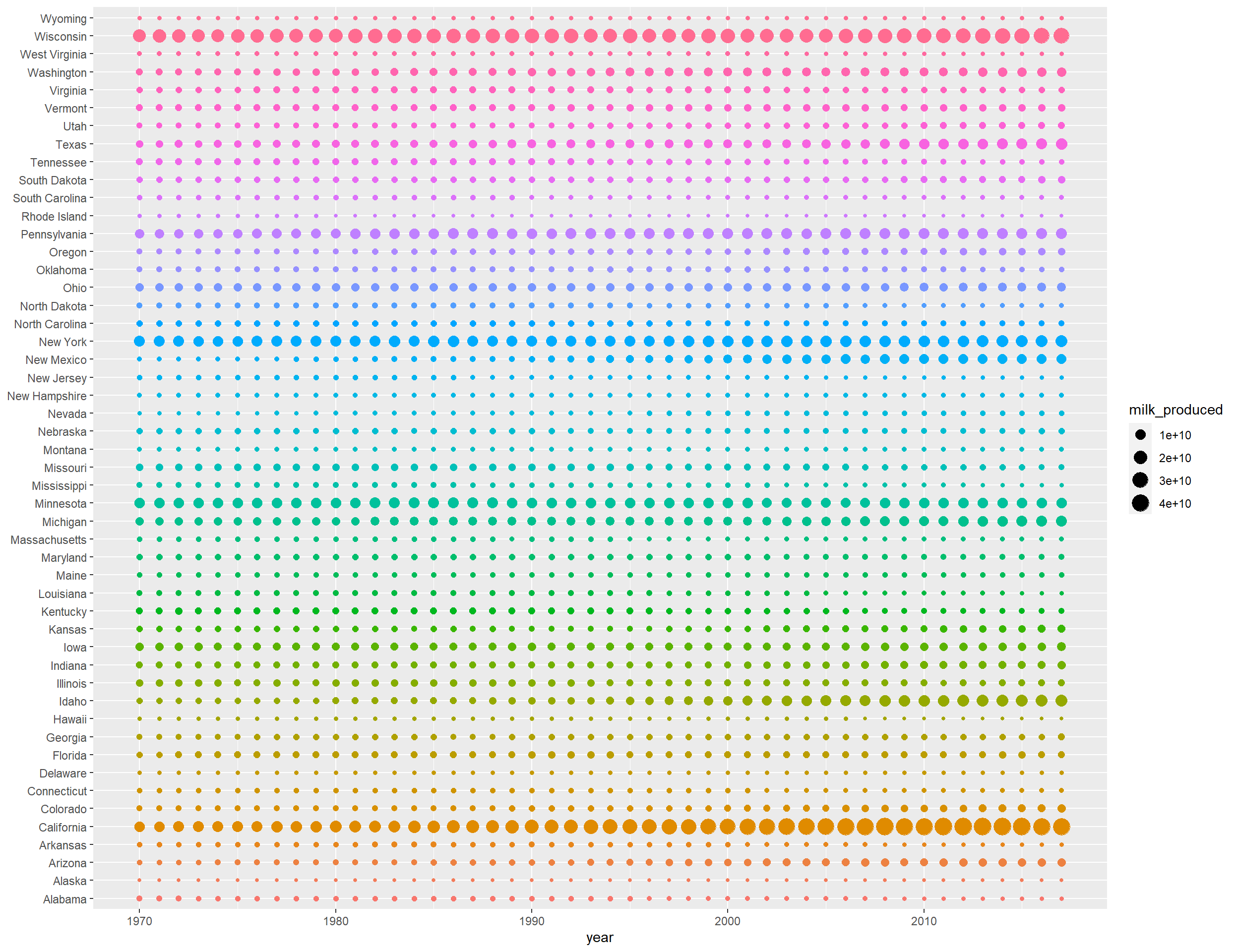
If you think the above plot is too fuzzy, the following heatmap is created to convey the same information.
state_milk %>%
  ggplot(aes(factor(year), state, fill = milk_produced)) +
  geom_tile() +
  scale_fill_gradient2(high = "red",
                       low = "white",
                       mid = "blue",
                       midpoint = mean(state_milk$milk_produced)) +
  labs(
    x = NULL,
    y = NULL,
    fill = "pounds of milk produced",
    title = "State-wise Milk Produced (pounds)"
  ) +
  scale_x_discrete(breaks = seq(1970, 2017, by = 3))