U.S. PhD Data Analysis with Extensive Data Cleaning/Processing

Sat, Oct 2, 2021 5-minute read

The data context of this blog post is interesting, as it is about PhD graduates in the U.S. from various years. As a Ph.D. student majoring in Data Science, this is revelant to me, although Data Science is not shown in the datasets.

The clean dataset is from TidyTuesday, and later I will use the raw datasets from NSF to carry out extensive data cleaning, which can shed some light on data preprocessing steps from the EXCEL files.

library(tidyverse)
library(patchwork)
library(readxl)

phd <- read_csv("https://raw.githubusercontent.com/rfordatascience/tidytuesday/master/data/2019/2019-02-19/phd_by_field.csv") %>%
  mutate(broad_field = str_to_title(broad_field),
         year = as.integer(year))


phd

## # A tibble: 3,370 x 5
##    broad_field   major_field                field                    year n_phds
##    <chr>         <chr>                      <chr>                   <int>  <dbl>
##  1 Life Sciences Agricultural sciences and~ Agricultural economics   2008    111
##  2 Life Sciences Agricultural sciences and~ Agricultural and horti~  2008     28
##  3 Life Sciences Agricultural sciences and~ Agricultural animal br~  2008      3
##  4 Life Sciences Agricultural sciences and~ Agronomy and crop scie~  2008     68
##  5 Life Sciences Agricultural sciences and~ Animal nutrition         2008     41
##  6 Life Sciences Agricultural sciences and~ Animal science, poultr~  2008     18
##  7 Life Sciences Agricultural sciences and~ Animal sciences, other   2008     77
##  8 Life Sciences Agricultural sciences and~ Environmental science    2008    182
##  9 Life Sciences Agricultural sciences and~ Fishing and fisheries ~  2008     52
## 10 Life Sciences Agricultural sciences and~ Food science             2008     96
## # ... with 3,360 more rows

p1 <- phd %>% 
  group_by(broad_field, year) %>%
  summarize(total_phd = sum(n_phds, na.rm = T)) %>%
  ungroup() %>%
  mutate(broad_field = fct_reorder(broad_field, -total_phd, sum)) %>%
  ggplot(aes(year, total_phd, color = broad_field)) +
  geom_line(size = 1) +
  scale_x_continuous(breaks = seq(2008, 2020)) +
  theme(
    plot.title = element_text(size = 18),
    axis.text = element_text(size = 13),
    axis.title = element_text(size = 15),
    legend.position = "top"
  ) +
  labs(x = NULL,
       y = "# of Ph.D.",
       color = "broad field",
       title = "# of Ph.D. across Various Broad Fields")

## `summarise()` has grouped output by 'broad_field'. You can override using the `.groups` argument.

p2 <- phd %>%
  group_by(year) %>% 
  summarize(total_phd = sum(n_phds, na.rm = T)) %>%
  ggplot(aes(year, total_phd)) +
  geom_line()  +
  scale_x_continuous(breaks = seq(2008, 2020)) +
  theme(
    plot.title = element_text(size = 18),
    axis.text = element_text(size = 13),
    axis.title = element_text(size = 15)
  ) +
  labs(x = NULL,
       y = "# of Ph.D.",
       color = "broad field",
       title = "Total # of Ph.D.")  

p2 / p1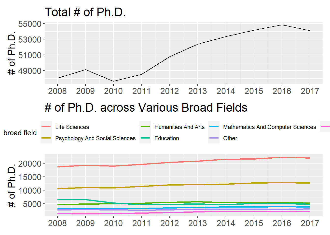

Analyzing The Raw Data

The following EXCEL files are downloaded from NSF, and they are Table 12, 13 and 14.

Doctorate recipients, by major field of study: Selected years, 1987–2017

major_field <- read_xlsx("sed17-sr-tab012.xlsx", skip = 3) %>%
  rename(field = 1)

major_field_processed <- major_field %>%
  pivot_longer(-field) %>%
  
  mutate(name = ifelse(str_detect(name, "\\.\\.\\."), NA, name)) %>%
  fill(name) %>% 
  drop_na() %>%
  rename(year = name, 
         num_of_phd = value) %>%
  mutate(year = as.numeric(year),
         num_of_phd = as.numeric(num_of_phd)) %>%
  filter(num_of_phd > 100) %>%
  mutate(field = ifelse(str_detect(field, "Other"), "Other", field),
         field = str_to_title(field))

major_field_processed %>% 
  filter(field != "All Fields") %>%
  complete(field, year, fill = list(0)) %>%
  ggplot(aes(year, field, fill = num_of_phd)) +
  geom_tile() +
  scale_fill_gradient2(low = "blue",
                       high = "red",
                       mid = "white",
                       midpoint = mean(major_field_processed$num_of_phd)) +
  scale_x_continuous(expand = c(0,0),
                     breaks = seq(1987, 2017, 2)) +
  theme(
    plot.title = element_text(size = 18),
    axis.text = element_text(size = 13)
  ) +
  labs(x = NULL,
       y = NULL,
       fill = "# of PhDs",
       title = "# of PhDs Produced by Various Fields")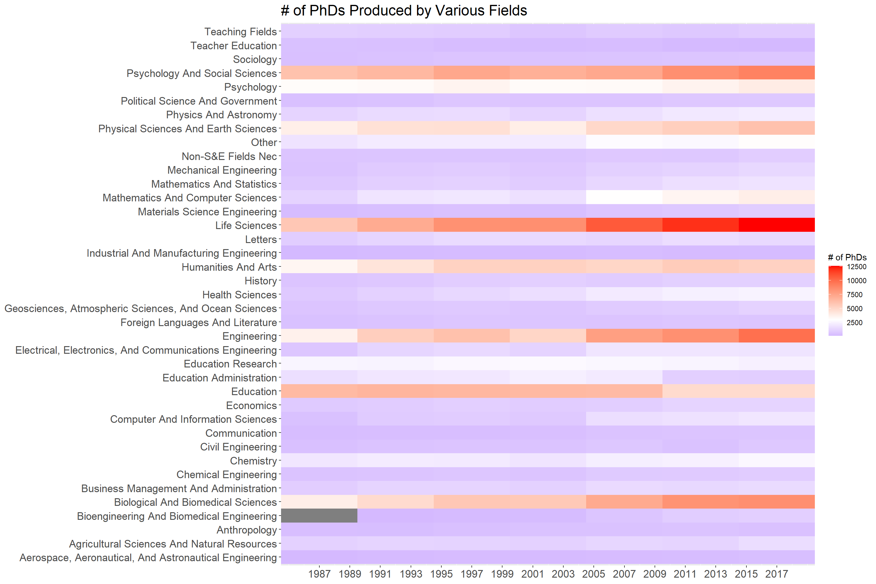

Doctorate recipients, by fine field of study: 2008–17

field <- read_xlsx("sed17-sr-tab013.xlsx", skip = 3) %>%
  rename(field = 1)

field_processed <- field %>%
  pivot_longer(-field, names_to = "year", values_to = "num_of_phds") %>%
  mutate(year = as.numeric(year),
         num_of_phds = as.numeric(num_of_phds))

top_7_fields <- field_processed %>%
  filter(field != "All fields")  %>%
  group_by(field) %>%
  summarize(total_num = sum(num_of_phds)) %>%
  arrange(desc(total_num)) %>%
  select(field) %>%
  head(7) %>%
  pull()

field_processed %>%
  filter(field %in% top_7_fields) %>%
  mutate(field = fct_reorder(field, -num_of_phds, sum)) %>%
  ggplot(aes(year, num_of_phds, color = field)) +
  geom_line(size = 1) +
  scale_x_continuous(breaks = seq(2008, 2020, by = 2)) +
  labs(x = NULL,
       y = "# of PhDs",
       title = "# of PhDs from Top 7 Majors",
       subtitle = "Top Majors are computed based on total # of PhDs")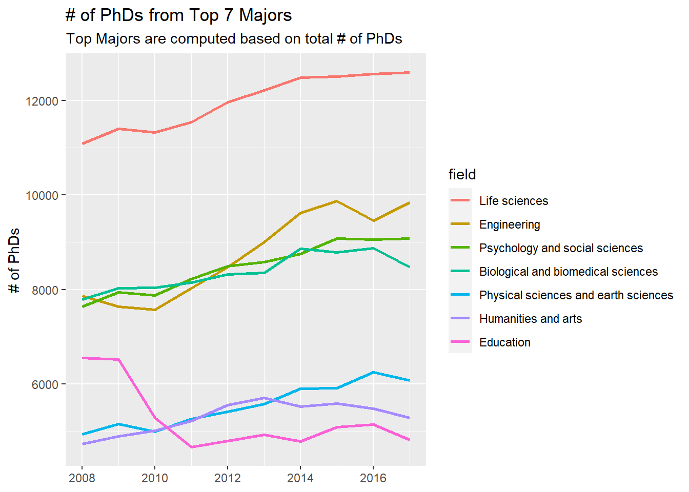

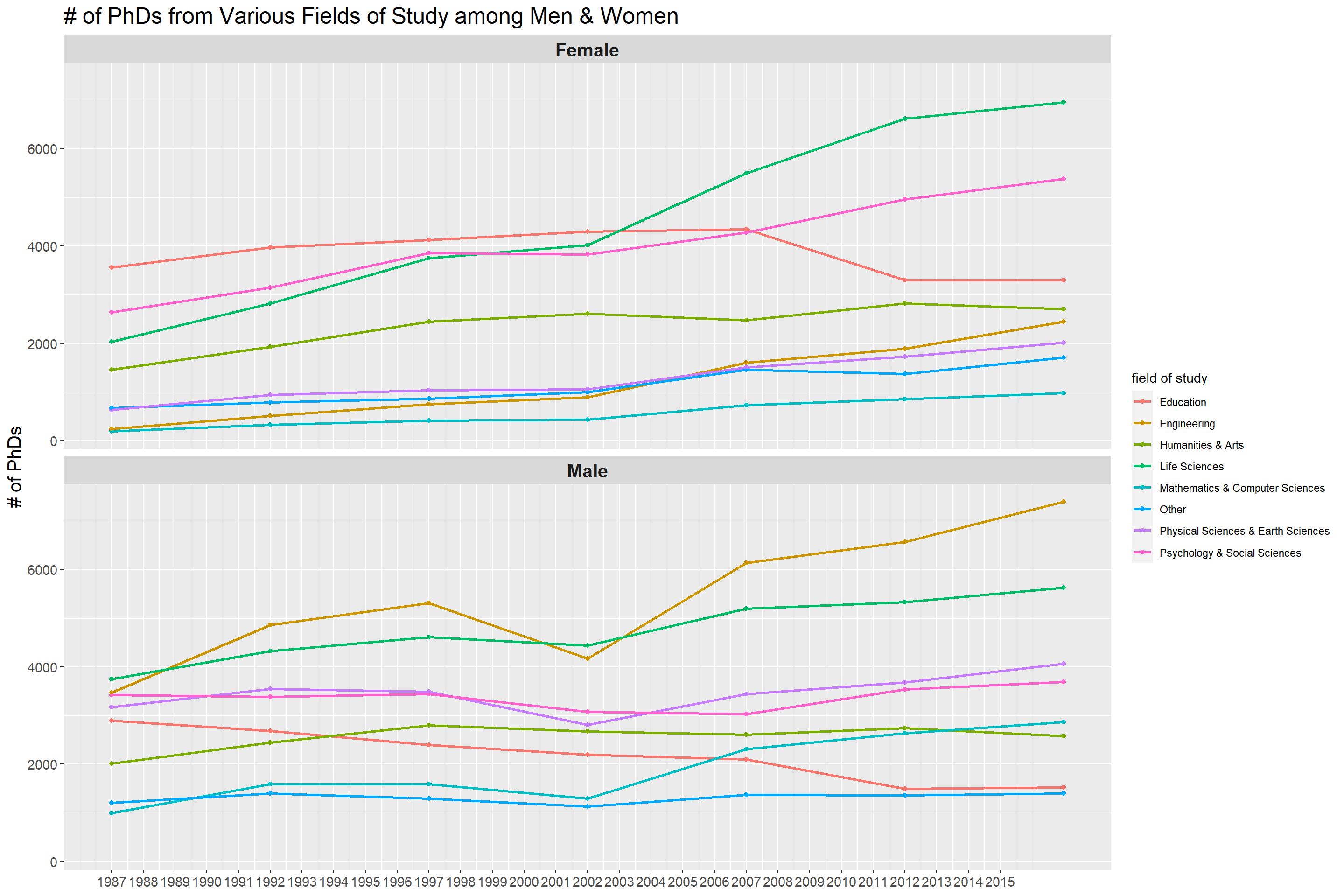
Doctorate recipients, by broad field of study and sex: Selected years, 1987–2017

field_gender <- read_xlsx("sed17-sr-tab014.xlsx", skip = 3) %>%
  rename(field = 1)

## New names:
## * `` -> ...3
## * `` -> ...5
## * `` -> ...7
## * `` -> ...9
## * `` -> ...11
## * ...

field_gender_processed <- field_gender %>%
  pivot_longer(-field, names_to = "year", values_to = "num_of_phds") %>% 
  mutate(year = ifelse(str_detect(year, "\\.\\.\\."), NA, year)) %>%
  fill(year) %>%
  drop_na() %>%
  mutate(year = as.numeric(year),
         num_of_phds = as.numeric(num_of_phds)) %>%
  filter(num_of_phds > 100)

fields_filtered <-field_gender_processed %>%
  filter(!field %in% c("Male", "Female")) %>%
  select(field) %>%
  distinct() %>%
  pull()


field_gender_processed %>%
  mutate(field_of_study = ifelse(field %in% fields_filtered, field, NA)) %>%
  fill(field_of_study) %>%
  rename(gender = field) %>%
  mutate(gender = ifelse(gender == field_of_study, "Total", gender)) %>%
  mutate(field_of_study = fct_recode(field_of_study, 
                                     "All field" = "All fieldsa",
                                     "Life sciences" = "Life sciencesb",
                                     "Other" = "Otherc")) %>%
  filter(gender != "Total",
         field_of_study != "All field") %>%
  mutate(field_of_study = fct_reorder(field_of_study, -num_of_phds, sum),
         field_of_study = str_to_title(field_of_study),
         field_of_study = str_replace(field_of_study, "And", "&")) %>%
  ggplot(aes(year, num_of_phds, color = field_of_study)) +
  geom_point() +
  geom_line(size = 1) +
  facet_wrap(~gender, ncol = 1) +
  theme(
    strip.text = element_text(size = 15, face = "bold"),
    plot.title = element_text(size = 18),
    axis.title = element_text(size = 15),
    axis.text = element_text(size = 11)
  ) +
  scale_x_continuous(breaks = seq(1987, 2015)) +
  labs(x = NULL,
       y = "# of PhDs",
       color = "field of study",
       title = "# of PhDs from Various Fields of Study among Men & Women")