Board Games Visualization & Lasso Analysis

Sat, Oct 9, 2021 4-minute read

This blog post is about visualizing and analyzing the board games dataset from R for Data Science online community TidyTuesday.

Load the packages and the dataset with some processing.

library(tidyverse)
library(tidytext)
library(glmnet)
library(Matrix)
library(broom)

board_games <- read_csv("https://raw.githubusercontent.com/rfordatascience/tidytuesday/master/data/2019/2019-03-12/board_games.csv") %>%
  filter(playing_time < 500)%>%
  mutate(decade = 10 * floor(year_published/10))

board_games

## # A tibble: 10,466 x 23
##    game_id description      image   max_players max_playtime min_age min_players
##      <dbl> <chr>            <chr>         <dbl>        <dbl>   <dbl>       <dbl>
##  1       1 Die Macher is a~ //cf.g~           5          240      14           3
##  2       2 Dragonmaster is~ //cf.g~           4           30      12           3
##  3       3 Part of the Kni~ //cf.g~           4           60      10           2
##  4       4 When you see th~ //cf.g~           4           60      12           2
##  5       5 In Acquire, eac~ //cf.g~           6           90      12           3
##  6       6 In the ancient ~ //cf.g~           6          240      12           2
##  7       7 In Cathedral, e~ //cf.g~           2           20       8           2
##  8       8 In this interes~ //cf.g~           5          120      12           2
##  9       9 Although referr~ //cf.g~           4           90      13           2
## 10      10 Elfenland is a ~ //cf.g~           6           60      10           2
## # ... with 10,456 more rows, and 16 more variables: min_playtime <dbl>,
## #   name <chr>, playing_time <dbl>, thumbnail <chr>, year_published <dbl>,
## #   artist <chr>, category <chr>, compilation <chr>, designer <chr>,
## #   expansion <chr>, family <chr>, mechanic <chr>, publisher <chr>,
## #   average_rating <dbl>, users_rated <dbl>, decade <dbl>

Separating `category` column

bg_category <- board_games %>%
  separate(category, into = c("c1", "c2"), sep = ",") %>% 
  pivot_longer(cols = c(c1, c2), names_to = "c", values_to = "category")%>% 
  filter(!is.na(category)) %>%
  mutate(category = fct_lump(category, 10),
         total_rating = average_rating * users_rated,
         decade = 10 * floor(year_published/10))

Weighted rating based on category and decade

bg_category %>%
  group_by(category, decade) %>%
  summarize(weighted_rating = sum(total_rating)/sum(users_rated)) %>%
  ungroup() %>%
  complete(category, decade, fill = list(weighted_rating = NA)) %>%
  ggplot(aes(decade, category, fill = weighted_rating)) +
  geom_tile() +
  scale_fill_gradient2(high = "blue",
                       low = "red",
                       mid = "white",
                       midpoint = 6) +
  scale_x_continuous(breaks = seq(1950, 2010, 10),
                     expand = c(0,0)) +
  scale_y_discrete(expand = c(0,0)) +
  theme(axis.ticks = element_blank(),
        axis.title = element_text(size = 15),
        axis.text = element_text(size = 13),
        plot.title = element_text(size = 18),
        plot.subtitle = element_text(size = 13)) +
  labs(fill = "weighted rating",
       title = "Board Game Weighted Rating by Category (1950s to 2010s)",
       subtitle = "Weighed rating is computed based on # of users rated and average rating for each game")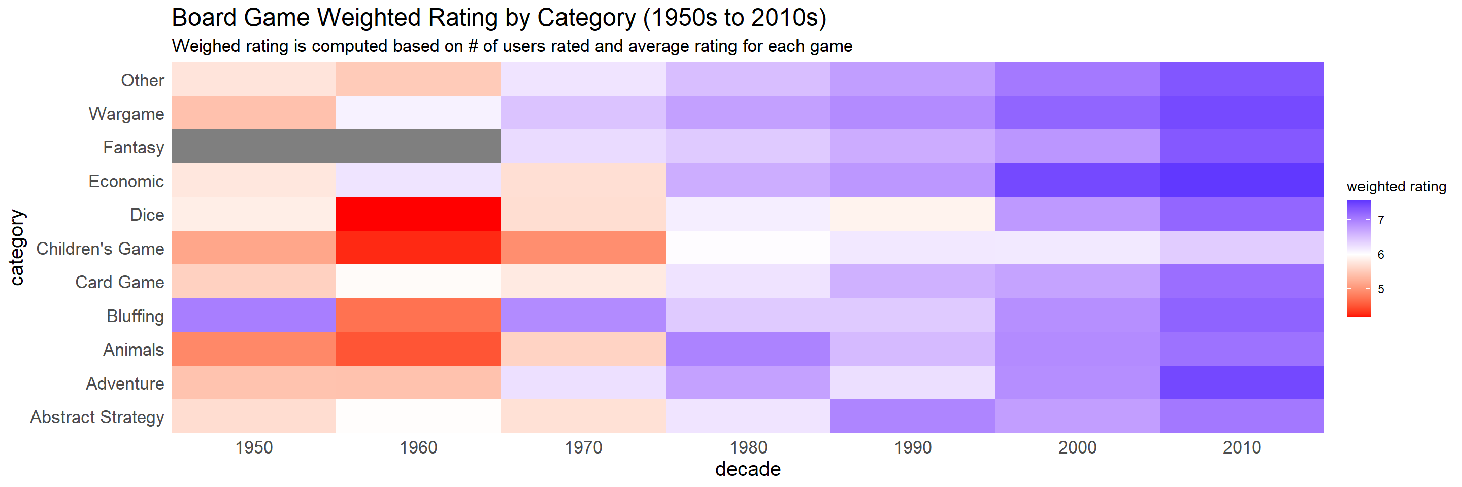

It seems like games from the recent decades received better ratings than their counterparts from 50s and 60s from all categories.

bg_category %>%
  mutate(decade = paste0(as.character(decade), "s"),
         category = reorder_within(category, playing_time, decade, median)) %>%
  ggplot(aes(playing_time, category, fill = category)) +
  geom_boxplot(show.legend = F) +
  facet_wrap(~decade, scales = "free_y") +
  scale_y_reordered() + 
  theme(
    strip.text = element_text(size = 15, face = "bold"),
    plot.title = element_text(size = 18),
    axis.title = element_text(size = 15),
    axis.text =element_text(size = 13)
  ) +
  labs(x = "playing time (mins)",
       title = "Board Game Playing Time across Various Categories (1950s - 2010s)")

Description text analysis

description_words <- board_games %>%
  mutate(decade = 10 * floor(year_published/10)) %>%
  select(description, decade) %>%
  unnest_tokens(word, description)%>%
  anti_join(stop_words) %>%
  filter(!str_detect(word, "[:digit:]"))

description_words_max <- description_words %>%
  group_by(decade) %>%
  count(word, name = "word_count_per_decade") %>%
  slice_max(word_count_per_decade, n = 10)
  
description_words_max %>% 
  mutate(word = reorder_within(word, word_count_per_decade, decade),
         decade = paste0(as.character(decade), "s")) %>%
  ggplot(aes(word_count_per_decade, word, fill = word)) +
  geom_col(show.legend = F) +
  facet_wrap(~decade, scales = "free") +
  scale_y_reordered() +
  theme(strip.text = element_text(size = 15, face = "bold"),
        axis.title = element_text(size = 15),
        axis.text = element_text(size = 13),
        plot.title = element_text(size = 18)) +
  labs(x = "# of words in game description",
       y = NULL,
       title = "Game Description Top 10 words (1950s - 2010s)")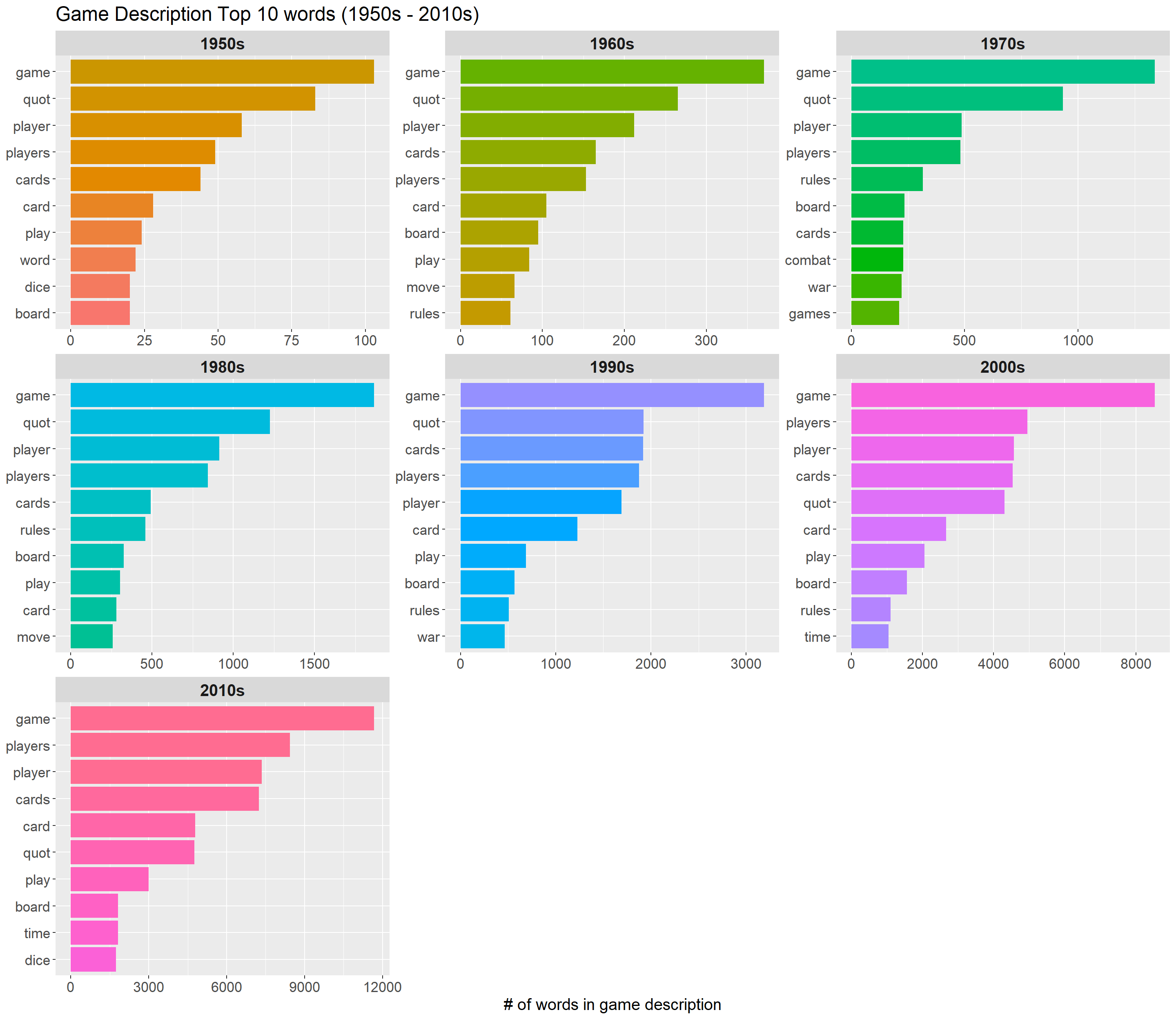

Lasso analysis

This section is inspired by David Robinson’s code

Processing categorical variables

bg_pivot <- board_games %>%
  select(game_id, name, family, category, artist, designer, publisher) %>%
  pivot_longer(-c(game_id, name), names_to = "type", values_to = "value") %>%
  # using separate_rows to remove characters after ","
  separate_rows(value, sep = ",")

Processing non-categorical variable

bg_pivot_non_categorical <- board_games %>%
  transmute(game_id,
            name,
            year_published,
            log10_max_players = log10(max_players + 1),
            log10_max_playtime = log10(max_playtime + 1)) %>%
  pivot_longer(-c(game_id, name), names_to = "feature", values_to = "value")

Binding categorical and non-categorical variables together

features <- bg_pivot %>%
  unite(feature, type, value, sep = ": ") %>%
  add_count(feature) %>%
  filter(n > 100) %>%
  mutate(value = 1) %>%
  bind_rows(bg_pivot_non_categorical)

Cross-validation Lasso

feature_matrix <- features %>%
  cast_sparse(game_id, feature, value)

matching_index <- match(rownames(feature_matrix), board_games$game_id)
ratings <- board_games$average_rating[matching_index]

lasso_model <- cv.glmnet(feature_matrix, ratings)
lasso_model$glmnet.fit %>%
  tidy() %>%
  filter(term != "(Intercept)",
         lambda == lasso_model$lambda.1se) %>%
  slice_max(abs(estimate), n = 50) %>%
  mutate(term = fct_reorder(term, estimate)) %>%
  ggplot(aes(estimate, term, fill = term)) +
  geom_col(show.legend = F) +
  labs(x = "estimate coefficient",
       y = NULL,
       title = "The 50 Terms with Largest Estimates (absolute value)",
       subtitle = "Based on a Lasso model with cross validation")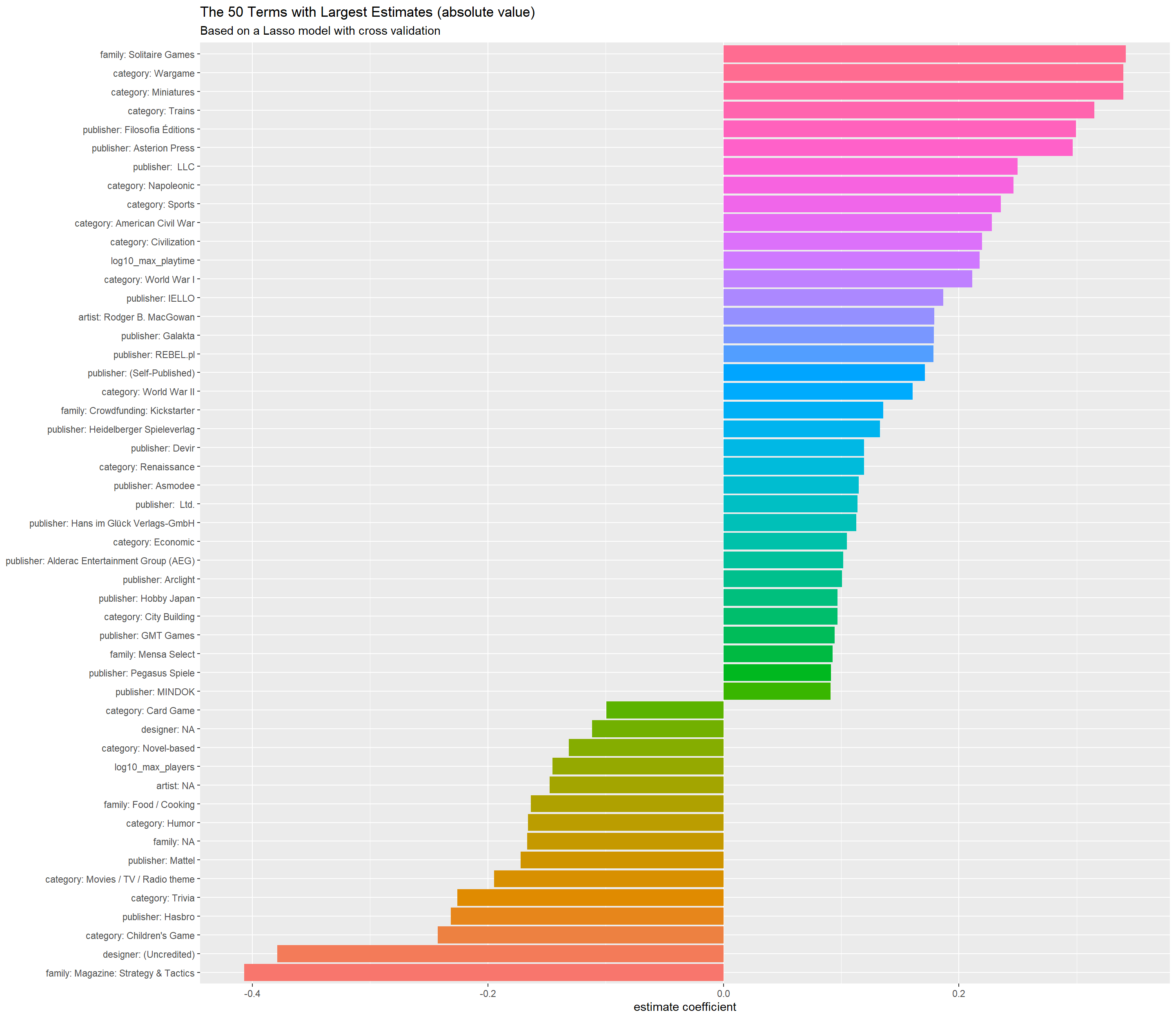

The bar chart above is very self-explanatory. category:Wargame would give the best rating. That is to say, if a board game’s category is Wargame, the rating will increase by roughly 0.3. But if it is about family and magazine with Strategy & Tactics, it would lower the rating most.