Seattle Bike Traffic Visualization with Functional Programming
This post analyzes the Seattle bike traffic dataset, which is interesting to visualize. It comes from TidyTuesday.
Load the packages and dataset with a few data processing steps.
library(tidyverse)
library(lubridate)
library(tidytext)
theme_set(theme_bw())
bike <- read_csv("https://raw.githubusercontent.com/rfordatascience/tidytuesday/master/data/2019/2019-04-02/bike_traffic.csv") %>%
mutate(date = mdy_hms(date),
year = year(date),
month = month(date),
day = day(date),
hour = hour(date),
weekday = wday(date, label = T, abbr = T, week_start = 1)) %>%
filter(bike_count < 1000) %>%
mutate(peak_hour = ifelse(hour > 7 & hour < 18, "Peak Hours", "Not Peak Hours"))
bike## # A tibble: 509,082 x 11
## date crossing direction bike_count ped_count year month day
## <dttm> <chr> <chr> <dbl> <lgl> <dbl> <dbl> <int>
## 1 2014-01-01 00:00:00 Broadwa~ North 0 NA 2014 1 1
## 2 2014-01-01 01:00:00 Broadwa~ North 3 NA 2014 1 1
## 3 2014-01-01 02:00:00 Broadwa~ North 0 NA 2014 1 1
## 4 2014-01-01 03:00:00 Broadwa~ North 0 NA 2014 1 1
## 5 2014-01-01 04:00:00 Broadwa~ North 0 NA 2014 1 1
## 6 2014-01-01 05:00:00 Broadwa~ North 0 NA 2014 1 1
## 7 2014-01-01 06:00:00 Broadwa~ North 0 NA 2014 1 1
## 8 2014-01-01 07:00:00 Broadwa~ North 0 NA 2014 1 1
## 9 2014-01-01 08:00:00 Broadwa~ North 2 NA 2014 1 1
## 10 2014-01-01 09:00:00 Broadwa~ North 0 NA 2014 1 1
## # ... with 509,072 more rows, and 3 more variables: hour <int>, weekday <ord>,
## # peak_hour <chr>Scan the dataset by using skim() from the skimr package.
skimr::skim(bike)| Name | bike |
| Number of rows | 509082 |
| Number of columns | 11 |
| _______________________ | |
| Column type frequency: | |
| character | 3 |
| factor | 1 |
| logical | 1 |
| numeric | 5 |
| POSIXct | 1 |
| ________________________ | |
| Group variables | None |
Variable type: character
| skim_variable | n_missing | complete_rate | min | max | empty | n_unique | whitespace |
|---|---|---|---|---|---|---|---|
| crossing | 0 | 1 | 9 | 40 | 0 | 7 | 0 |
| direction | 0 | 1 | 4 | 5 | 0 | 4 | 0 |
| peak_hour | 0 | 1 | 10 | 14 | 0 | 2 | 0 |
Variable type: factor
| skim_variable | n_missing | complete_rate | ordered | n_unique | top_counts |
|---|---|---|---|---|---|
| weekday | 0 | 1 | TRUE | 7 | Thu: 72960, Wed: 72859, Fri: 72710, Sat: 72696 |
Variable type: logical
| skim_variable | n_missing | complete_rate | mean | count |
|---|---|---|---|---|
| ped_count | 407072 | 0.2 | 0.25 | FAL: 76869, TRU: 25141 |
Variable type: numeric
| skim_variable | n_missing | complete_rate | mean | sd | p0 | p25 | p50 | p75 | p100 | hist |
|---|---|---|---|---|---|---|---|---|---|---|
| bike_count | 0 | 1 | 11.74 | 23.04 | 0 | 0 | 3 | 12 | 794 | ▇▁▁▁▁ |
| year | 0 | 1 | 2015.90 | 1.45 | 2013 | 2015 | 2016 | 2017 | 2019 | ▇▇▇▇▆ |
| month | 0 | 1 | 6.35 | 3.50 | 1 | 3 | 6 | 9 | 12 | ▇▅▅▅▇ |
| day | 0 | 1 | 15.74 | 8.79 | 1 | 8 | 16 | 23 | 31 | ▇▇▇▇▆ |
| hour | 0 | 1 | 11.50 | 6.92 | 0 | 6 | 12 | 18 | 23 | ▇▇▆▇▇ |
Variable type: POSIXct
| skim_variable | n_missing | complete_rate | min | max | median | n_unique |
|---|---|---|---|---|---|---|
| date | 0 | 1 | 2013-12-18 | 2019-02-28 23:00:00 | 2016-04-23 01:00:00 | 45572 |
bike %>%
  filter(!is.na(ped_count))
## # A tibble: 102,010 x 11
## date crossing direction bike_count ped_count year month day
## <dttm> <chr> <chr> <dbl> <lgl> <dbl> <dbl> <int>
## 1 2019-02-28 23:00:00 Burke G~ North 0 FALSE 2019 2 28
## 2 2019-02-28 22:00:00 Burke G~ North 0 FALSE 2019 2 28
## 3 2019-02-28 21:00:00 Burke G~ North 2 FALSE 2019 2 28
## 4 2019-02-28 20:00:00 Burke G~ North 2 TRUE 2019 2 28
## 5 2019-02-28 19:00:00 Burke G~ North 6 FALSE 2019 2 28
## 6 2019-02-28 04:00:00 Burke G~ North 0 FALSE 2019 2 28
## 7 2019-02-28 03:00:00 Burke G~ North 1 FALSE 2019 2 28
## 8 2019-02-28 02:00:00 Burke G~ North 0 FALSE 2019 2 28
## 9 2019-02-28 01:00:00 Burke G~ North 0 FALSE 2019 2 28
## 10 2019-02-28 00:00:00 Burke G~ North 0 FALSE 2019 2 28
## # ... with 102,000 more rows, and 3 more variables: hour <int>, weekday <ord>,
## # peak_hour <chr>ped_count is a column for pedestrain counts, but I am confused why it is a logical column.
bike %>%
  mutate(crossing = reorder_within(crossing, bike_count, peak_hour, median, na.rm = T)) %>%
  ggplot(aes(bike_count, crossing, fill = crossing)) +
  geom_boxplot(show.legend = F) +
  facet_wrap(~peak_hour, ncol = 1, scales = "free_y") +
  scale_y_reordered() +
  theme(
    strip.text = element_text(size = 15, face = "bold"),
    plot.title = element_text(size = 18),
    plot.subtitle = element_text(size = 13),
    axis.title = element_text(size = 14),
    axis.text = element_text(size = 13)
  ) +
  labs(
    x = "bike count",
    y = "Street Intersection",
    title = "Bike Count at Each Street during Peak and Non-peak Hours",
    subtitle = "Peak hours are between 7AM to 6 PM, and non-peak hours otherwise"
  )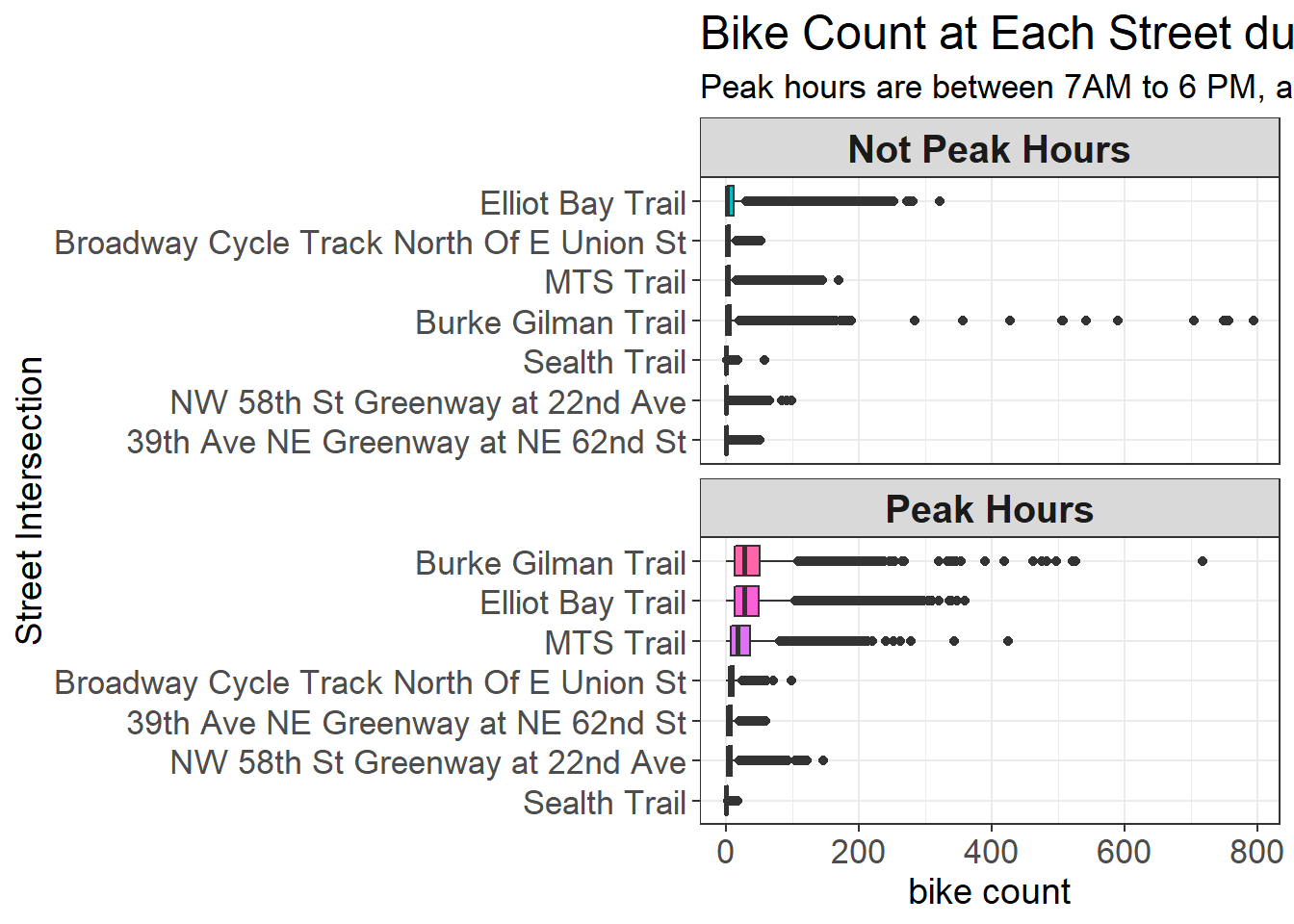
Storytelling: Bike count during non-peak hour is smaller on all crossings. A reasonable explanation is that people are commuting to work during peak hours (7AM - 6PM).
Weekday Average Bike Count
bike %>%
group_by(weekday, crossing, direction) %>%
summarize(avg_count = mean(bike_count, na.rm = T)) %>%
ggplot(aes(weekday, crossing, fill = avg_count)) +
geom_tile() +
facet_wrap(~direction, scales = "free") +
scale_fill_gradient2(
high = "red",
low = "green",
mid = "white",
midpoint = 10
) +
scale_x_discrete(expand = c(0,0))+
scale_y_discrete(expand = c(0,0)) +
theme(
strip.text = element_text(size = 15, face = "bold"),
plot.title = element_text(size = 18),
axis.title = element_text(size = 14),
axis.text = element_text(size = 13)
) +
labs(
x = NULL,
y = "Street Intersection",
fill = "average bike count",
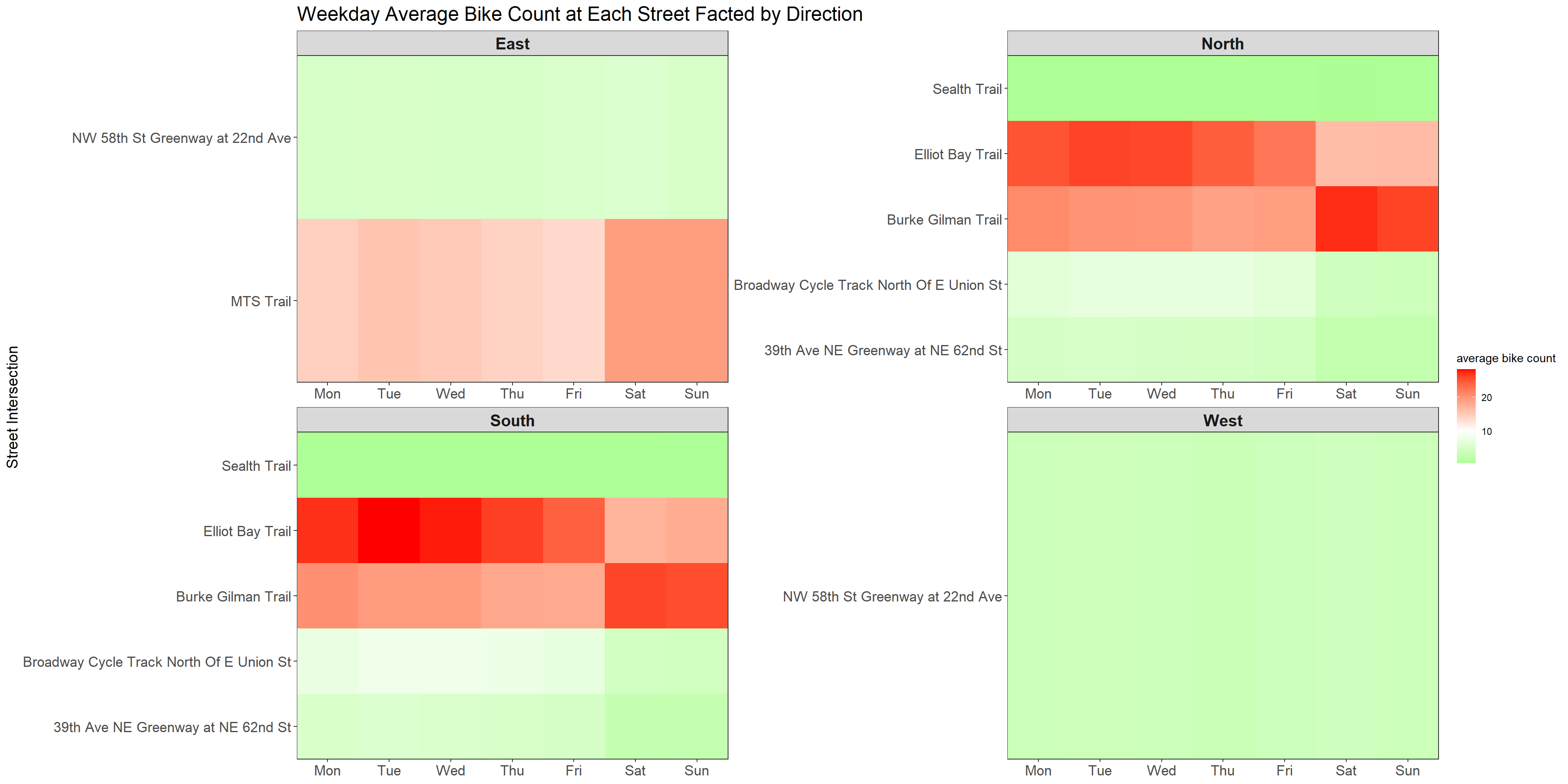
title = "Weekday Average Bike Count at Each Street Facted by Direction"
)
North & South Direction Commute
bike %>%
  filter(direction %in% c("North", "South")) %>%
  group_by(crossing, direction, hour) %>%
  summarize(total_bike = sum(bike_count)) %>%
  mutate(bike_pct = total_bike/sum(total_bike)) %>%
  ggplot(aes(hour, total_bike, color = direction)) +
  geom_line(size = 1) +
  facet_wrap(~crossing, ncol = 1, scales = "free") +
  #scale_y_continuous(label = percent) +
  scale_x_continuous(breaks = seq(0,23,2)) +
  labs(y = "# of bikes at the crossing in this hour",
       x = "hour",
       title = "Which Direction Does People Commute?") +
  theme(
    strip.text = element_text(size = 15, face = "bold"),
    plot.title = element_text(size = 18)
  )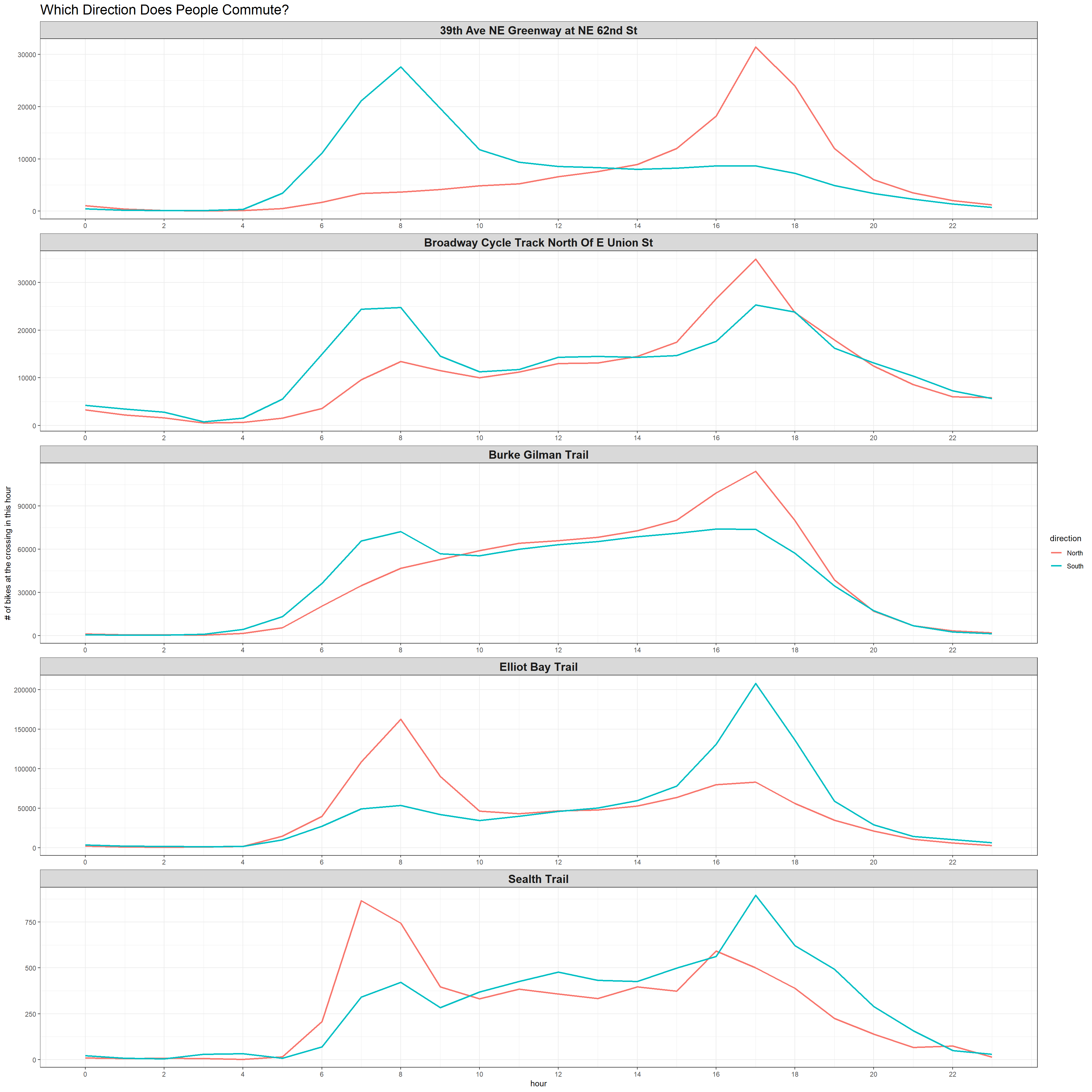
It is interesting to note that if a certain direction is peaked during the morning commute hours, the opposite direction will be peaked during the evening commute hours.
Yearly Street Intersection Hourly Average Bike Count
hourly_bike_heatmap <- function(year_index){
  bike %>%
    group_by(year, hour, crossing) %>%
    summarize(avg_count = mean(bike_count, na.rm = T)) %>%
    ungroup() %>%
    filter(year == year_index) %>%
    ggplot(aes(hour, crossing, fill = avg_count)) +
    geom_tile()+
    scale_fill_gradient2(
      high = "red",
      low = "green",
      mid = "white",
      midpoint = 15
    ) +
    scale_x_continuous(expand = c(0,0), breaks = seq(0, 23))+
    scale_y_discrete(expand = c(0,0)) +
    theme(
      strip.text = element_text(size = 15, face = "bold"),
      plot.title = element_text(size = 18),
      axis.title = element_text(size = 14),
      axis.text = element_text(size = 13)
    )+
    labs(
      y = "Street Intersection",
      fill = "average bike count",
      title = paste(year_index, "Street Intersection Hourly Average Bike Count")
    )
}

map(sort(unique(bike$year))[2:7], hourly_bike_heatmap)
## [[1]]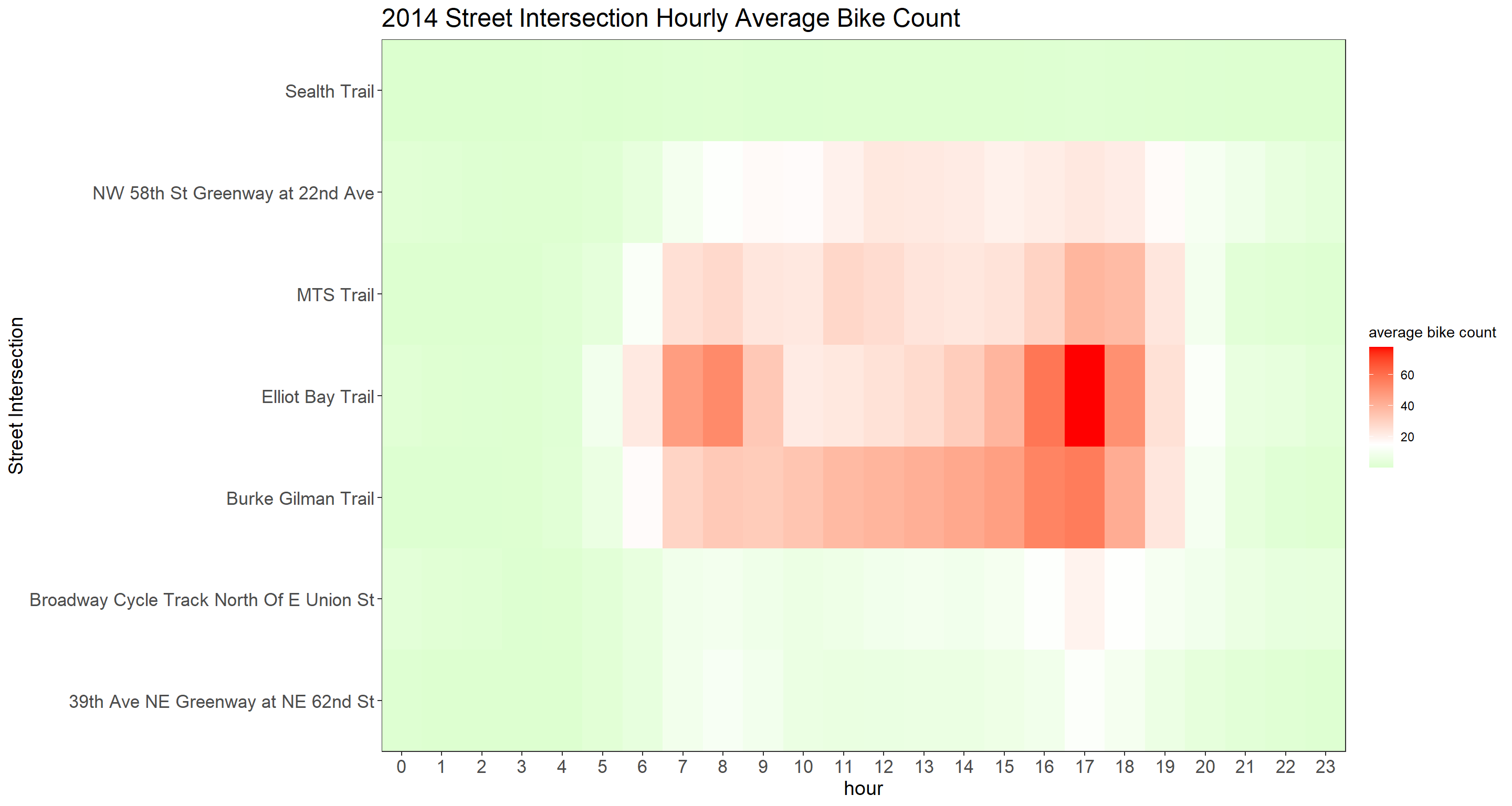
##
## [[2]]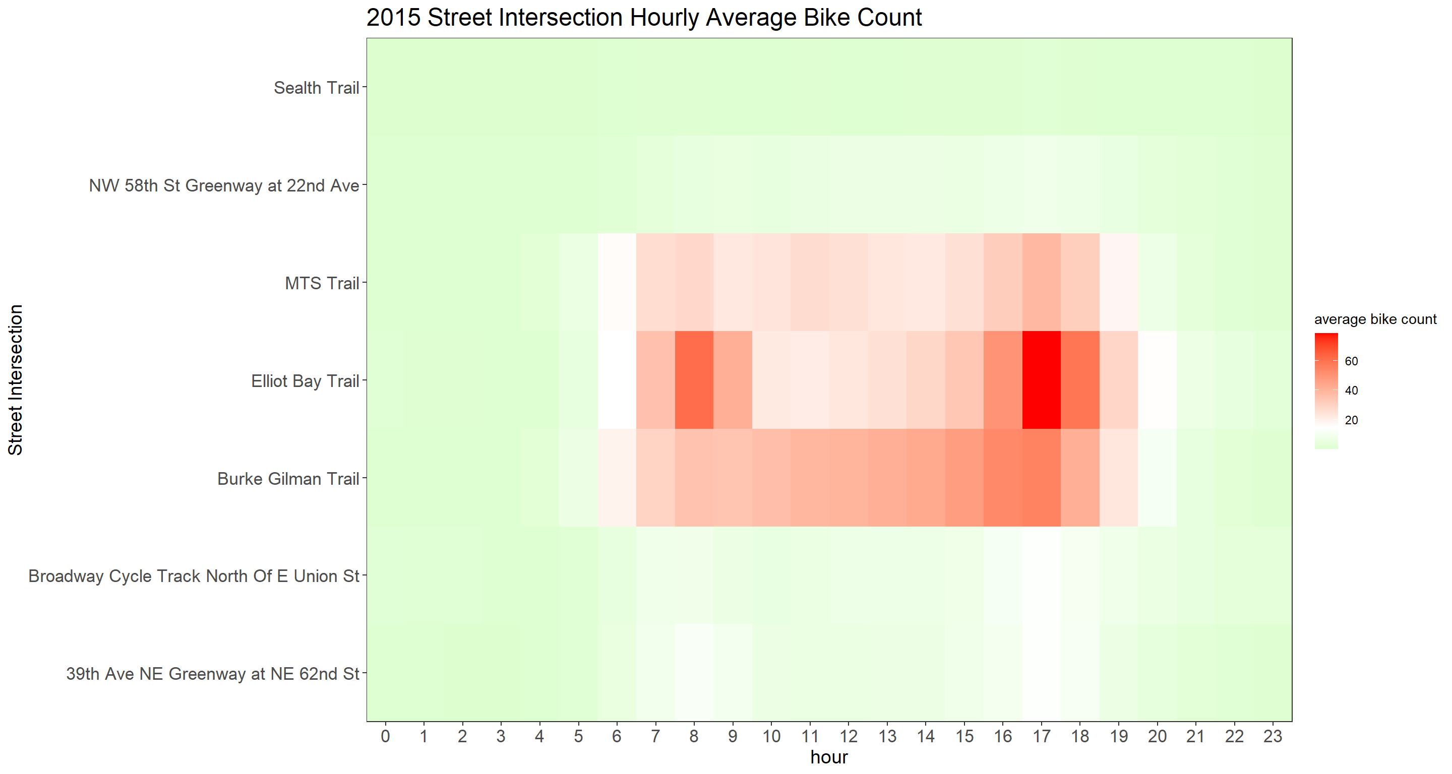
##
## [[3]]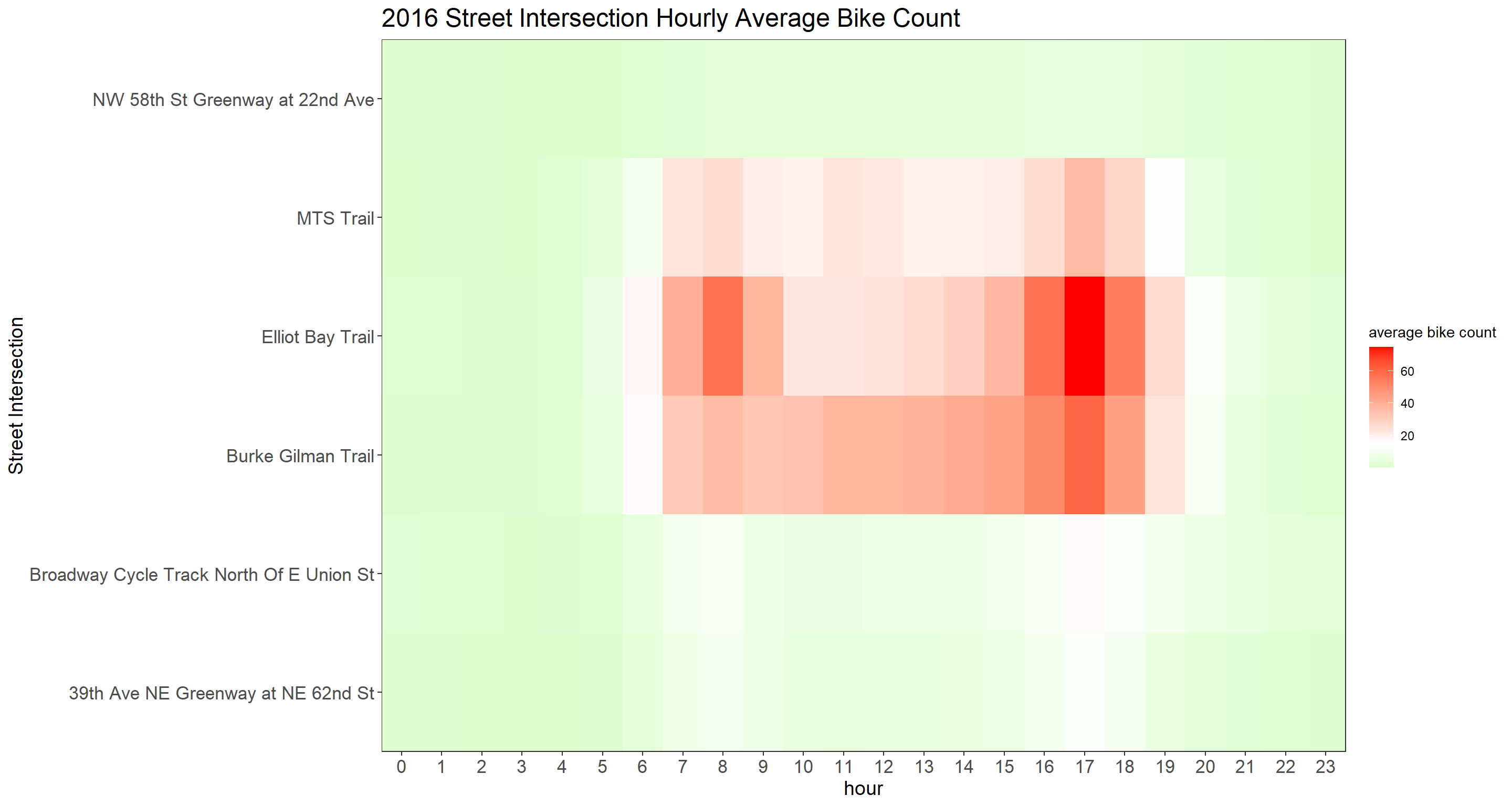
##
## [[4]]
##
## [[5]]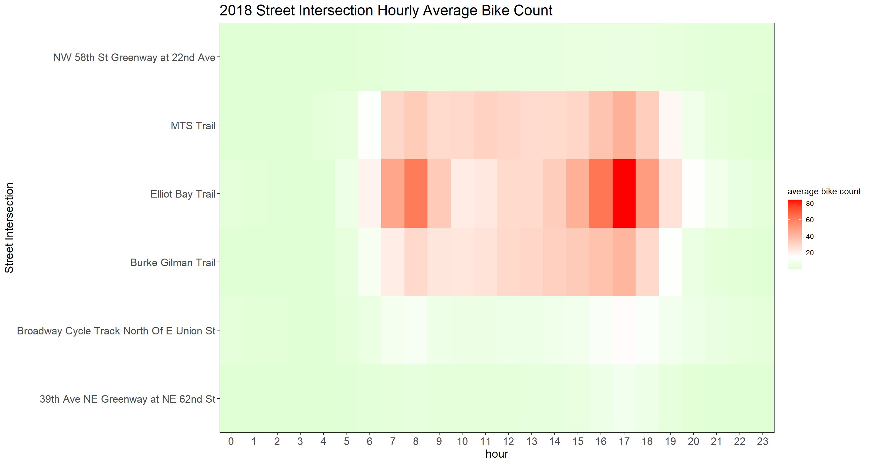
##
## [[6]]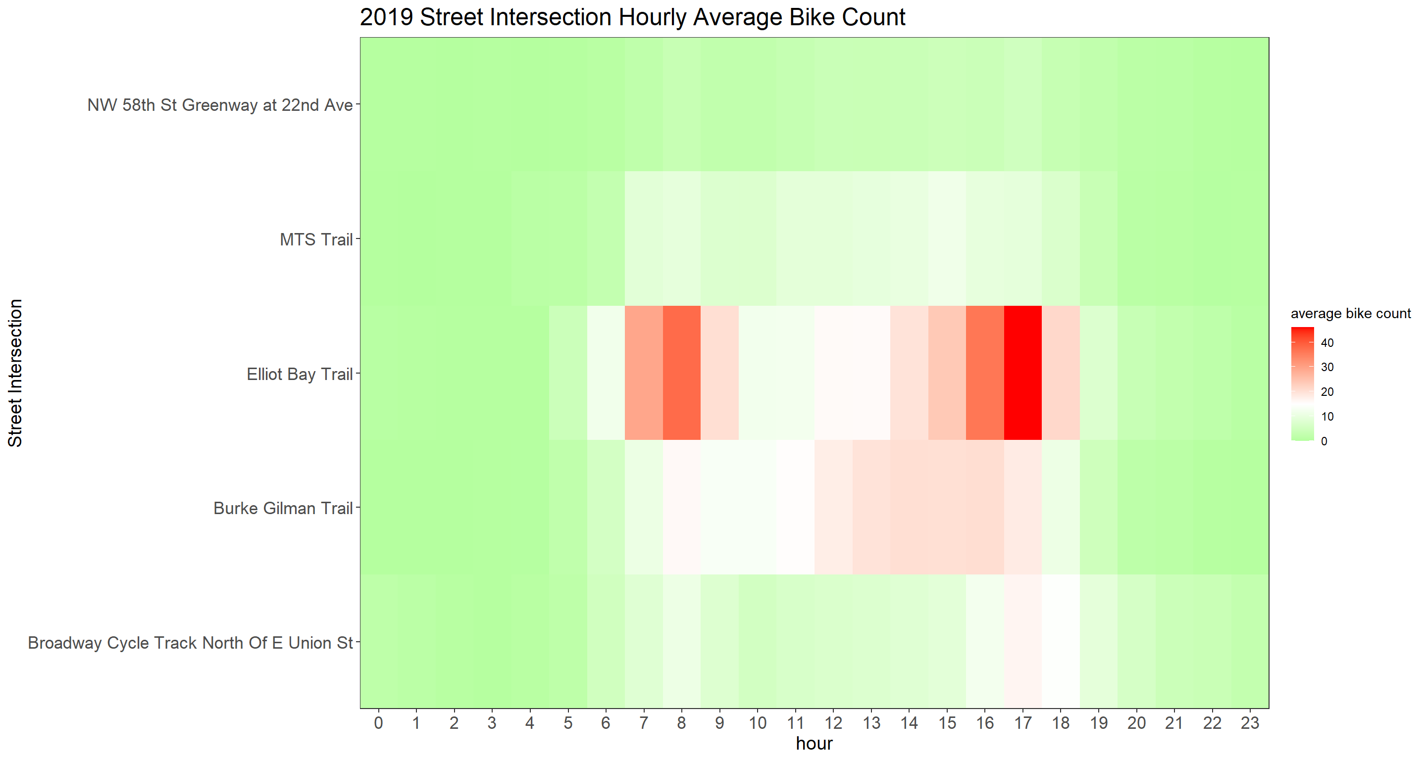
hourly_bike_heatmap <- function(year_index){
  bike %>%
    group_by(year, month, crossing) %>%
    summarize(avg_count = mean(bike_count, na.rm = T)) %>%
    ungroup() %>%
    filter(year == year_index) %>%
    complete(month, crossing, fill = list(avg_count = 0)) %>%
    ggplot(aes(month, crossing, fill = avg_count)) +
    geom_tile()+
    scale_fill_gradient2(
      high = "red",
      low = "green",
      mid = "white",
      midpoint = 15
    ) +
    scale_x_continuous(expand = c(0,0), breaks = seq(0, 23))+
    scale_y_discrete(expand = c(0,0)) +
    theme(
      strip.text = element_text(size = 15, face = "bold"),
      plot.title = element_text(size = 18),
      axis.title = element_text(size = 14),
      axis.text = element_text(size = 13)
    )+
    labs(
      y = "Street Intersection",
      fill = "average bike count",
      title = paste(year_index, "Street Intersection Hourly Average Bike Count")
    )
}

map(sort(unique(bike$year))[2:7], hourly_bike_heatmap)
## [[1]]
##
## [[2]]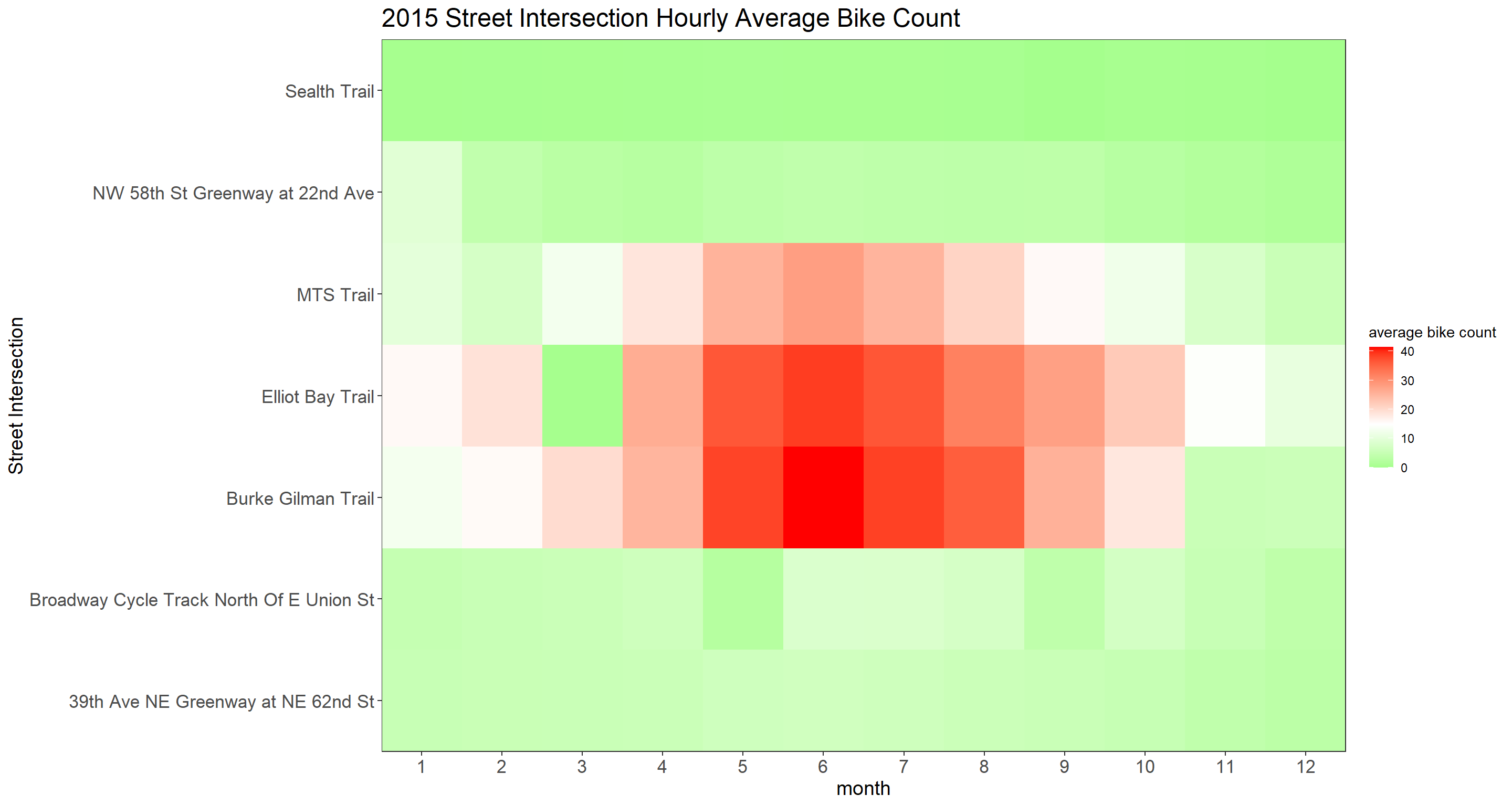
##
## [[3]]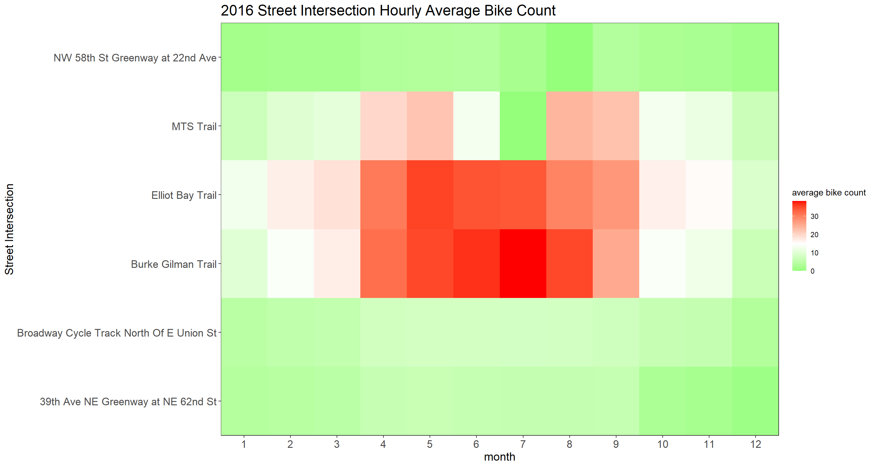
##
## [[4]]
##
## [[5]]
##
## [[6]]