Chicago Bird Collisions with Bootstraps

Yearly Collisions

bird_collisions %>%
  mutate(year = year(date)) %>%
  count(year, flight_call) %>%
  mutate(flight_call = fct_reorder(flight_call, -n, sum)) %>%
  ggplot(aes(year, n, color = flight_call)) +
  geom_line(size = 1) +
  scale_x_continuous(breaks = seq(1980, 2015, 5)) +
  labs(x = NULL,
       y = "Total Collision Count",
       color = "flight call",
       title = "Yearly Total Collision Count")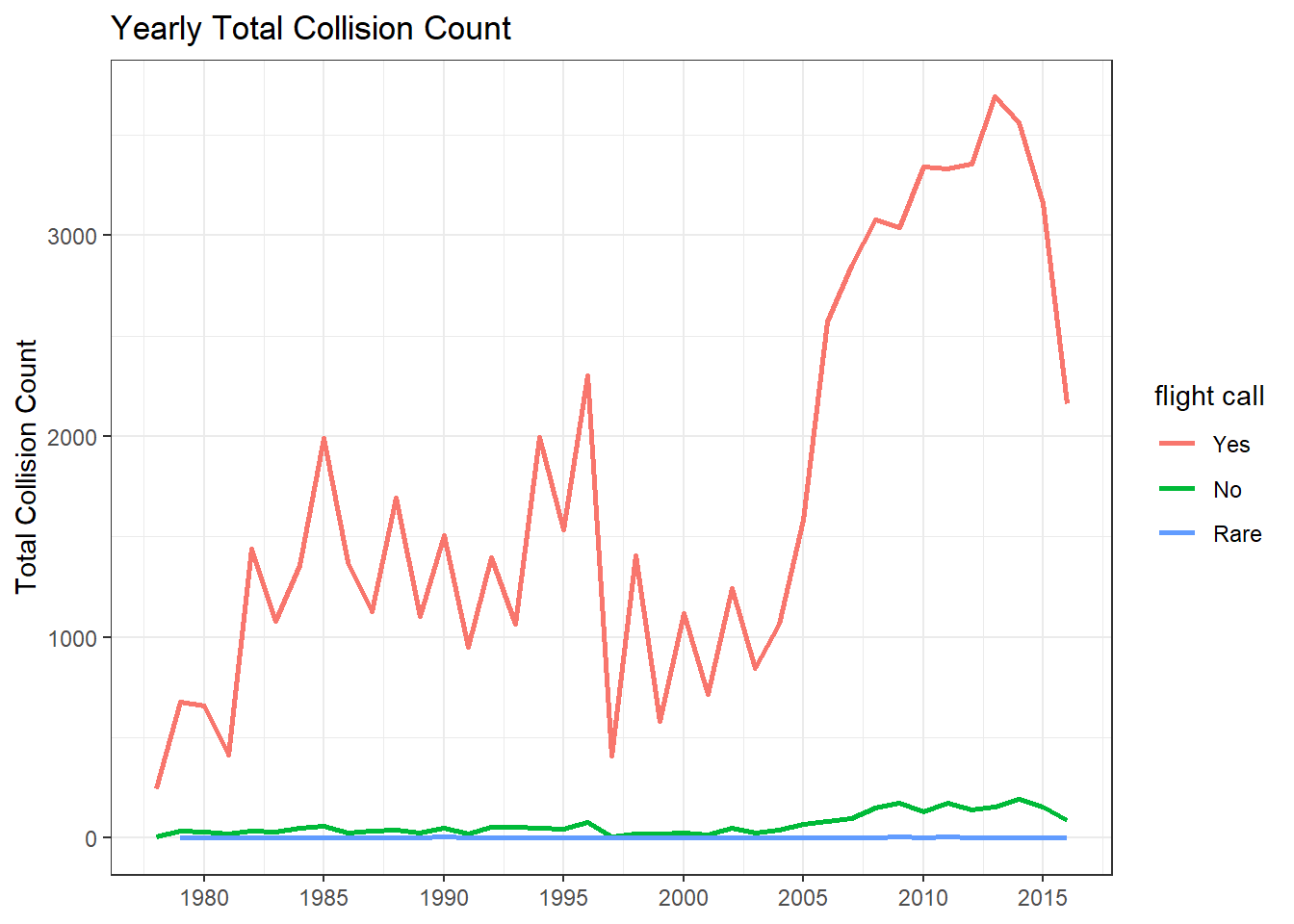 

A significant number of collisions were having flight call involved, and the count was peaked around 2013.

Monthly Collisions

bird_collisions %>%
  mutate(month = month(date, label = T)) %>%
  count(month) %>%
  ggplot(aes(n, month, fill = month)) +
  geom_col(show.legend = F) +
  labs(x = "count",
       y = NULL,
       title = "Total Monthly Bird Collision Counts") +
  theme(
    axis.title = element_text(size = 13),
    axis.text = element_text(size = 12),
    plot.title = element_text(size = 18)
  )

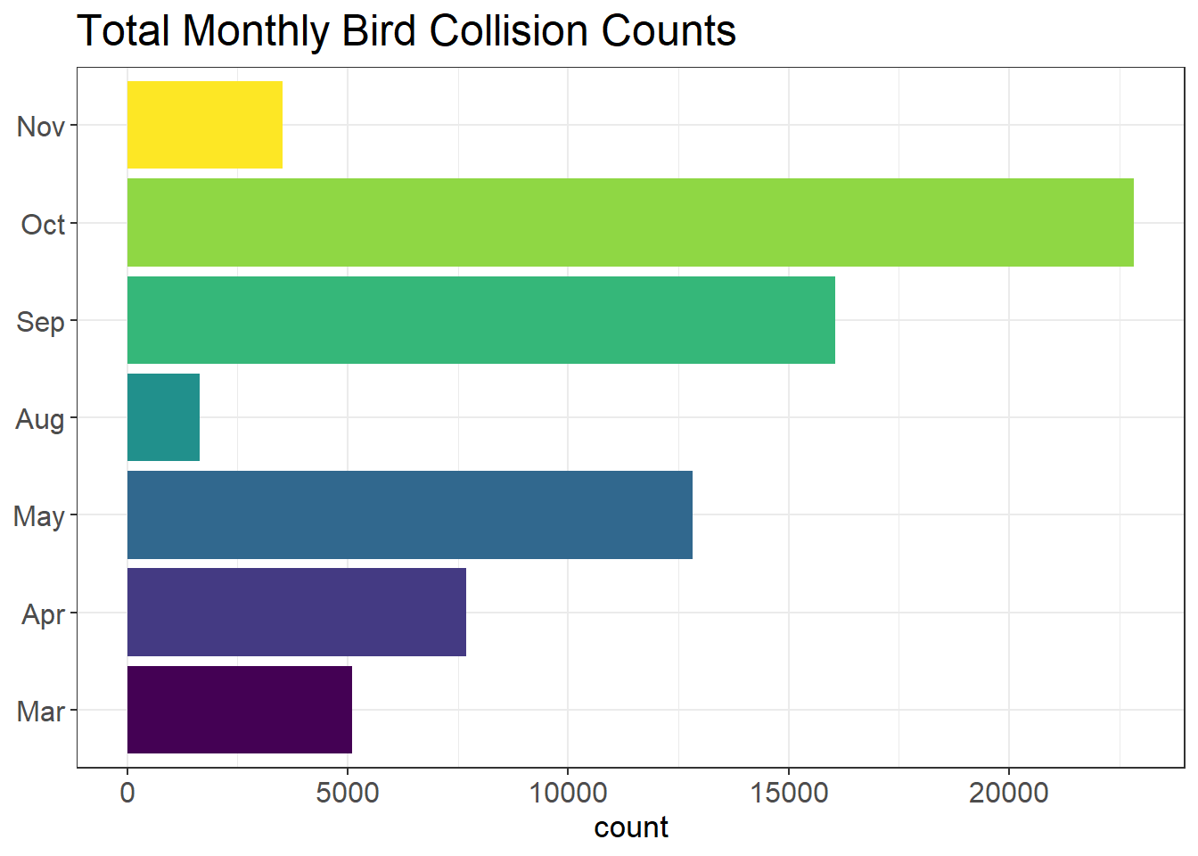
October was the month that most of the collision took place, but August was the least.

bird_collisions %>%
  count(genus, habitat, sort = T) %>%
  mutate(genus = fct_reorder(genus, n, sum)) %>%
  ggplot(aes(n, genus, fill = habitat)) +
  geom_col() +
  labs(
    x = "collision count",
    title = "Collision Counts Among All Genera Filled by Habitat"
  )

Melospiza had the largest number of collisions and its habitat preference was Edge and Open, although Edge was slightly more popular.

bird_collisions %>%
  count(locality, family, sort = T) %>%
  ggplot(aes(locality, family, fill = n)) +
  geom_tile() +
  scale_fill_gradient2(
    high = "red",
    low = "green",
    mid = "white",
    midpoint = 10000
  ) +
  scale_x_discrete(expand = c(0,0)) +
  scale_y_discrete(expand = c(0,0)) +
  labs(
    fill = "collision count",
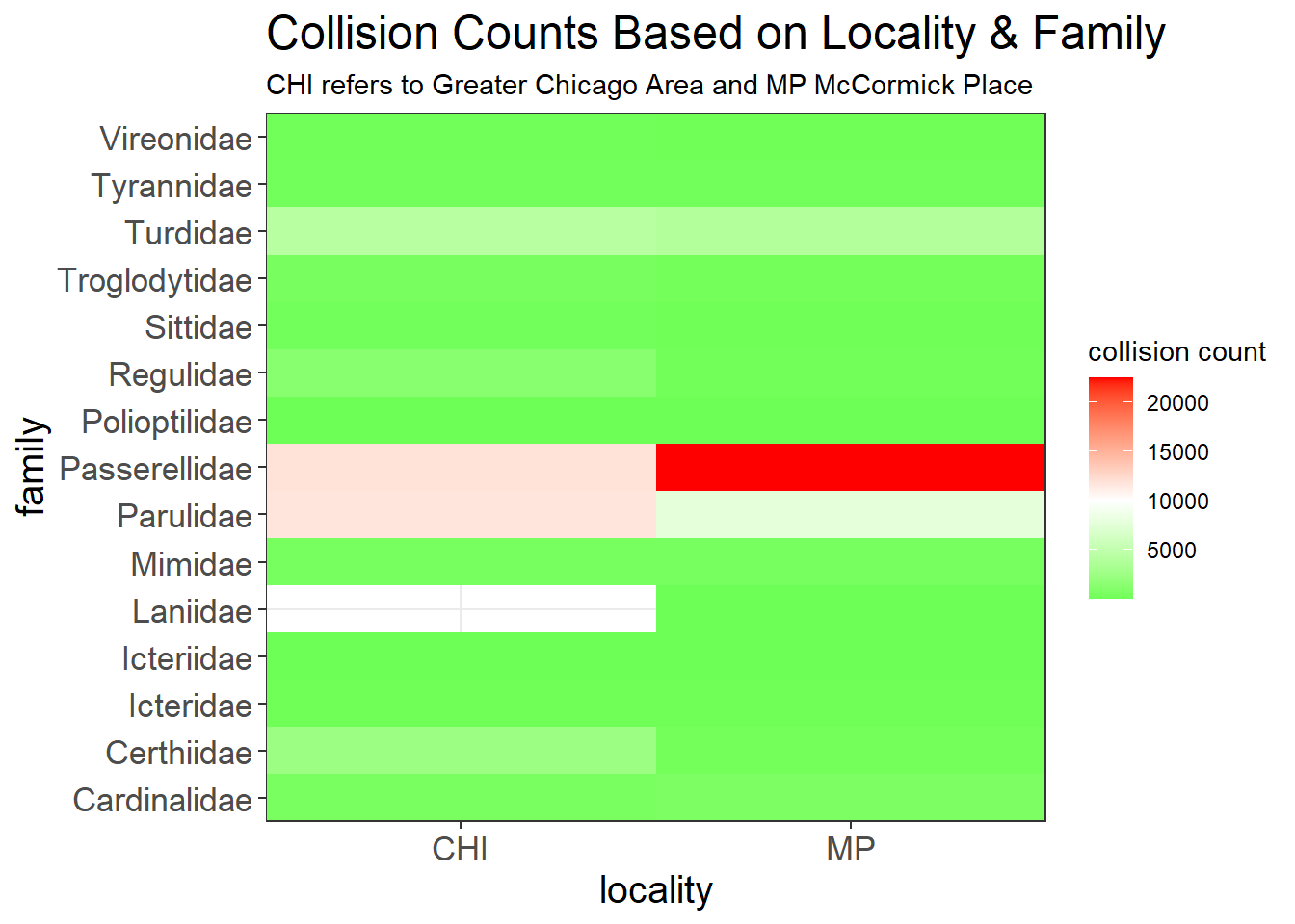
    title = "Collision Counts Based on Locality & Family",
    subtitle = "CHI refers to Greater Chicago Area and MP McCormick Place"
  ) +
  theme(
    plot.title = element_text(size = 18),
    axis.title = element_text(size = 15),
    axis.text = element_text(size = 13)
  )

bird_collisions %>%
  mutate(species = fct_lump(species, n = 30)) %>%
  count(species, stratum, sort = T) %>%
  filter(species != "Other") %>%
  mutate(species = fct_reorder(species, n, sum)) %>%
  ggplot(aes(n, species, fill = stratum)) +
  geom_col() +
  labs(
    x = "collision count",
    title = "Top 30 Collision Counts Based on Species & Stratum"
  ) +
  theme(
    plot.title = element_text(size = 18),
    axis.title = element_text(size = 15),
    axis.text = element_text(size = 13)
  )

The most deadly bird species was Albicollis.

Light Score

mp_light  %>%
  group_by(date) %>%
  summarize(total_ls = sum(light_score)) %>%
  mutate(year = year(date),
         month = month(date, label = T)) %>%
  ggplot(aes(total_ls, month, fill = month)) +
  geom_col(show.legend = F) +
  facet_wrap(~year) +
  labs(x = "total light score",
       y = NULL,
       title = "Total Light Score from each Year and Month") +
  theme(
    plot.title = element_text(size = 18),
    strip.text = element_text(size = 15),
    axis.text.x = element_text(angle = 90, size = 13),
    axis.text.y = element_text(size = 13),
    axis.title = element_text(size = 15)
  )

There was a total light score decrease after the year of 2008, but from the line plot made in the first place, the number of bird collisions was peaked around 2013, which did not have a high light score.

Bootstraps

This is my first time using bootstraps from rsample package, and the following code is mostly copied from Daivd Robinson’s github repo with some minor changes for learning purposes (here is the link).

by_day_mp <- bird_collisions %>%
  left_join(mp_light, by = "date") %>%
  filter(!is.na(light_score)) %>%
  group_by(date, locality) %>%
  summarize(collisions = n()) %>%
  ungroup() %>%
  complete(date, locality, fill = list(collisions = 0)) %>%
  right_join(mp_light %>% crossing(locality = c("CHI", "MP")), by = c("date", "locality")) %>%
  filter(date <= "2016-11-13") %>% 
  replace_na(list(collisions = 0)) %>%
  mutate(locality = ifelse(locality == "CHI", "Greater Chicago", "McCormick Place"))

geom_mean <- function(x) {
  exp(mean(log(x + 1)) - 1)
}

bootstrap_cis <- by_day_mp %>%
  bootstraps(times = 1000) %>% 
  # David's code does not work here, so I aded model and unnest(model)
  mutate(bootstrap_tibble = map(splits, as_tibble)) %>%
  unnest(bootstrap_tibble) %>%
  group_by(light_score, locality, id) %>%
  summarize(avg_collisions = geom_mean(collisions)) %>%
  summarize(bootstrap_low = quantile(avg_collisions, .025),
            bootstrap_high = quantile(avg_collisions, .975))

by_day_mp %>%
  group_by(light_score, locality) %>%
  summarize(avg_collisions = geom_mean(collisions),
            nights = n()) %>%
  ggplot(aes(light_score, color = locality)) +
  geom_line(aes(y = avg_collisions)) +
  geom_ribbon(aes(ymin = bootstrap_low, ymax = bootstrap_high),
              data = bootstrap_cis,
              alpha = .25) +
  expand_limits(y = 0) +
  labs(x = "Light score at McCormick place (higher means more lights on)",
       y = "Geometric mean of the number of collisions",
       title = "Brighter lights at McCormick place correlate with more bird collisions there, and not with Chicago overall",
       subtitle = "Ribbon shows 95% bootstrapped percentile confidence interval",
       color = "")