Data Visualization on Nobel Prize Winners
Sun, Oct 31, 2021
4-minute read
Nobel Prize is a world-class prize. In this blog post, the prize winners’ information and prize category will be analyzed. The datasets are from the TidyTuesday Project, which is a wonderful online data science learning community for R users.
Load the packages and the datasets!
library(tidyverse)
library(scales)
library(lubridate)
library(WDI)
library(countrycode)
winner_all_pubs <- read_csv("https://raw.githubusercontent.com/rfordatascience/tidytuesday/master/data/2019/2019-05-14/nobel_winner_all_pubs.csv") %>%
mutate(journal = str_to_title(journal),
affiliation = str_to_title(affiliation),
category = str_to_title(category))
winners <- read_csv("https://raw.githubusercontent.com/rfordatascience/tidytuesday/master/data/2019/2019-05-14/nobel_winners.csv")winner_all_pubs %>%
group_by(laureate_id, category) %>%
summarize(total_publication = n(),
prize_publication = sum(is_prize_winning_paper == "YES")) %>%
mutate(prize_ratio = prize_publication / total_publication) %>%
ungroup() %>%
ggplot(aes(prize_ratio, category, fill = category)) +
geom_violin(show.legend = F) +
scale_x_continuous(labels = percent) +
labs(x = "prize paper ratio",
title = "Category-wise Prize Paper Ratio",
subtitle = "prize paper ratio between # of winning papers and total # of papers")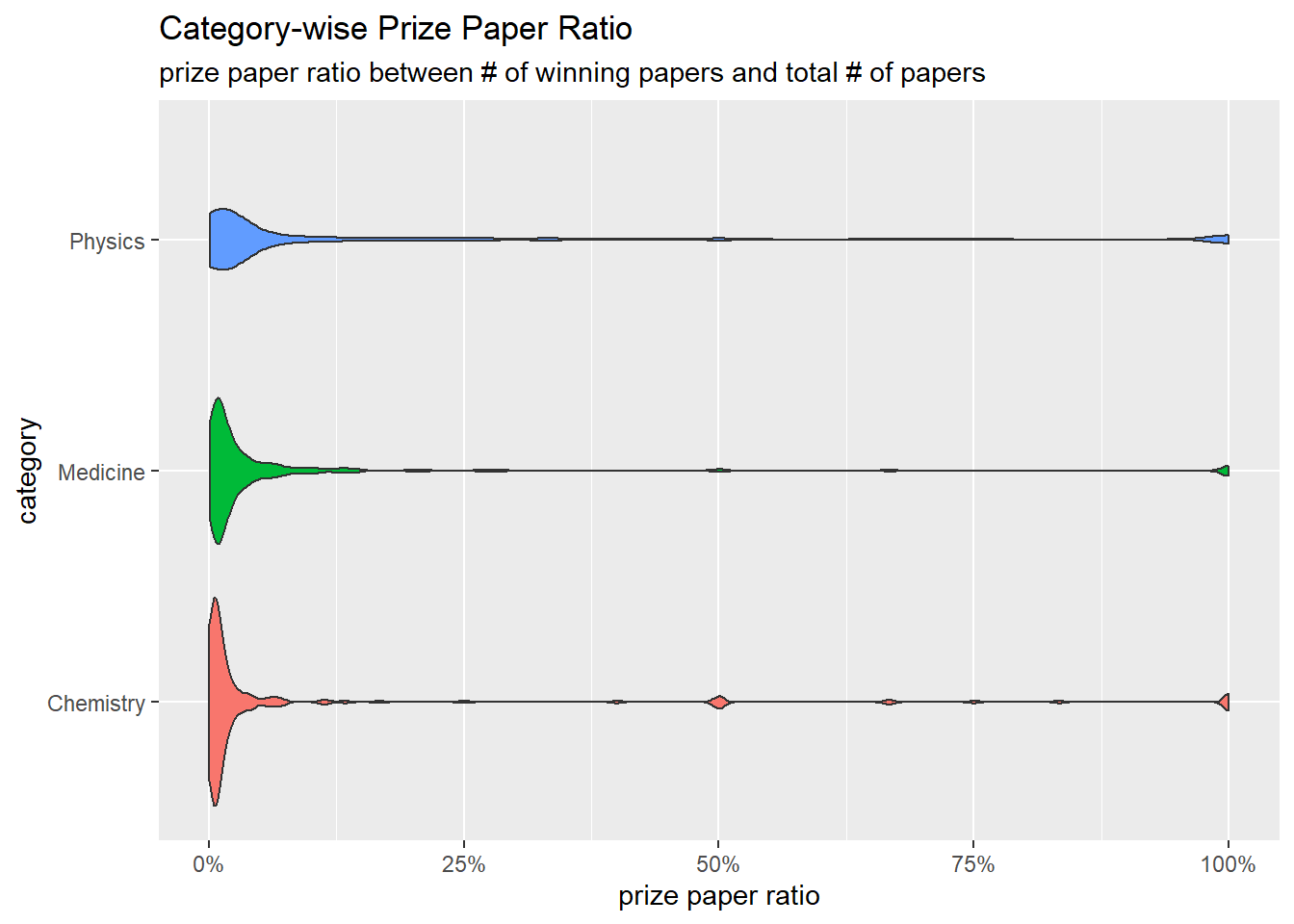
winning_papers <- winner_all_pubs %>%
  filter(is_prize_winning_paper == "YES")


winning_papers %>%
  mutate(wait_year = prize_year - pub_year) %>%
  filter(wait_year > 0) %>%
  ggplot(aes(wait_year, category, fill = category)) +
  geom_boxplot(show.legend = F) +
  scale_x_continuous() +
  labs(x = "wait year",
       title = "How many years did paper publication need to wait to get the Nobel Prize?",
       subtitle = "Wait year is defined as prize year minus paper publication year")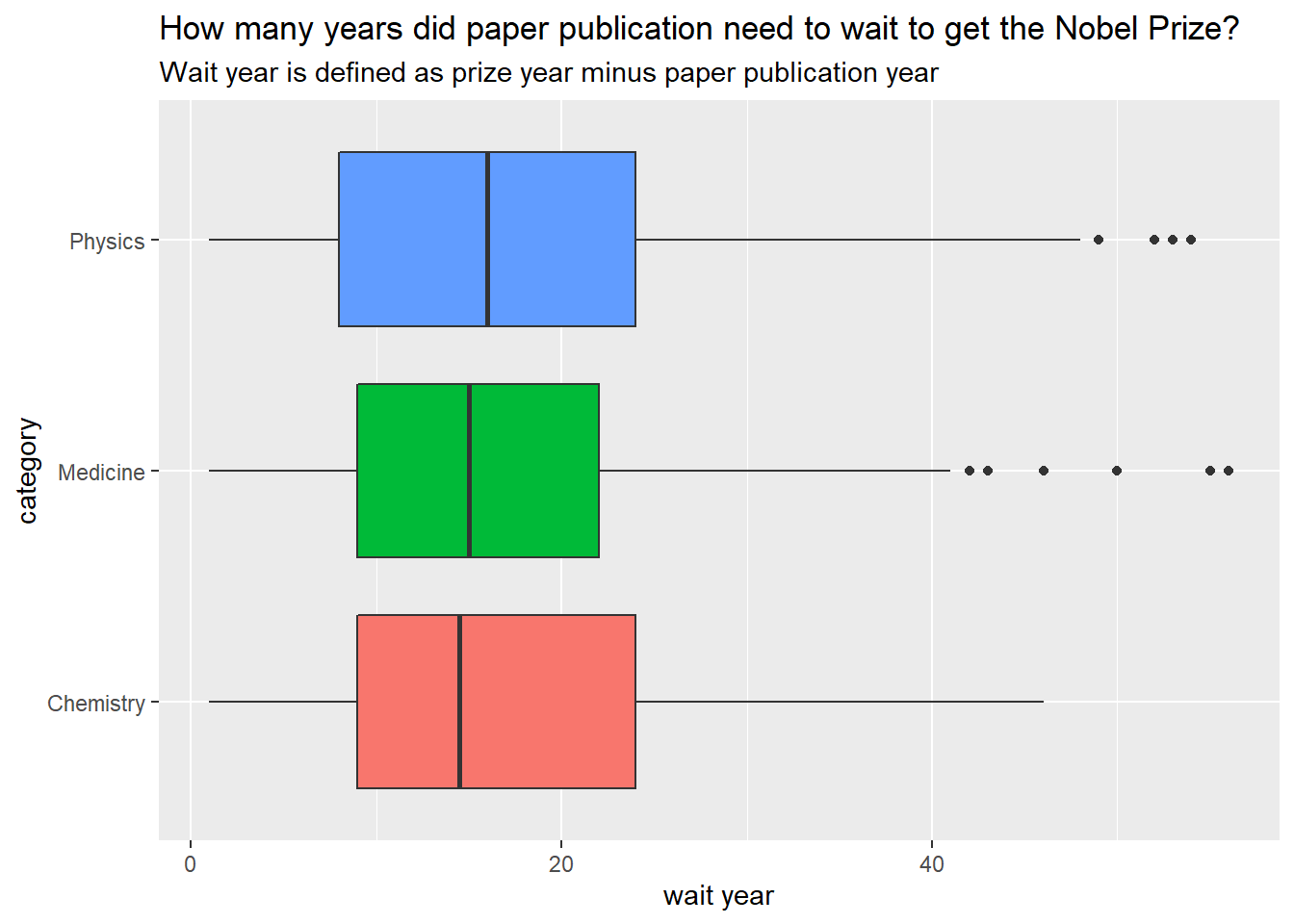
Wait median of 10+ years to win the nobel prize after paper publication!
Which paper is the winning paper for the winner?
winner_all_pubs %>%
  mutate(pub_decade = 10 * floor(pub_year/10)) %>%
  group_by(laureate_name) %>%
  mutate(pub_rank = rank(pub_year, ties.method = "first"),
         total_pub = n()) %>%
  filter(is_prize_winning_paper == "YES") %>%
  mutate(winning_percentage = pub_rank / total_pub) %>%
  group_by(category, pub_decade) %>%
  summarize(avg_win = mean(winning_percentage)) %>%
  ggplot(aes(pub_decade, avg_win, color = category)) +
  geom_line(size = 1) +
  labs(x = "decade",
       y = "average winning paper rank in the winner's career",
       title = "The Average Winning Paper Rank in each Decade")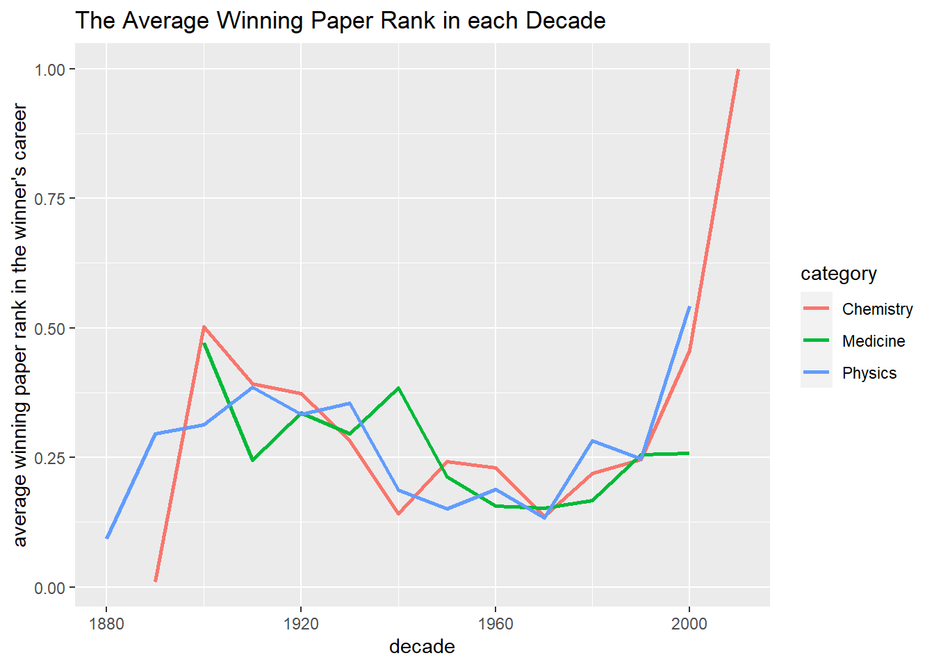
Publication Journals
winner_all_pubs %>%
  group_by(journal, category) %>%
  summarize(winning_paper_count = sum(is_prize_winning_paper == "YES"),
            total_paper = n())  %>%
  filter(winning_paper_count > 0,
         total_paper > 5,
         !is.na(journal)) %>%
  mutate(ratio = winning_paper_count / total_paper) %>%
  arrange(desc(ratio)) %>%
  ungroup() %>%
  mutate(journal = fct_lump(journal, n = 10, w = ratio)) %>%
  filter(journal != "Other") %>%
  mutate(journal = fct_reorder(journal, ratio)) %>%
  ggplot(aes(ratio, journal, fill = category)) +
  geom_col() +
  scale_x_continuous(labels = percent) +
  labs(x = "winning ratio",
       title = "Top 10 Winning Journals with the Highest Winning Ratio")
winners %>%
  mutate(birth_year = year(birth_date),
         prize_age = prize_year - birth_year,
         category = fct_reorder(category, prize_age, median, na.rm = T)) %>%
  ggplot(aes(prize_age, category, fill = category)) +
  geom_boxplot(show.legend = F) +
  labs(x = "age when awarded the Nobel Prize",
       title = "Nobel Laureate Age When Receiving the Prize") +
  theme(
    axis.title = element_text(size = 15),
    axis.text = element_text(size = 13),
    plot.title = element_text(size = 18)
  )
When Nobel Prize winners’ birth country and winning country are same
same_country <- winners %>%
  filter(birth_country == organization_country)


same_country %>%
  count(birth_country, category, sort = T) %>%
  mutate(birth_country = fct_reorder(birth_country, n, sum)) %>%
  ggplot(aes(n, birth_country, fill = category)) +
  geom_col()
When Nobel Prize winners’ birth country and winning country are different
diff_country <- winners %>%
  filter(birth_country != organization_country)

diff_country %>%
  count(birth_country, organization_country, sort = T) %>%
  group_by(organization_country) %>%
  summarize(total = sum(n)) %>%
  ungroup() %>%
  mutate(organization_country = fct_reorder(organization_country, total)) %>%
  ggplot(aes(total, organization_country, fill = organization_country)) +
  geom_col(show.legend = F) +
  labs(x = "total # of the prize winners born outside of the country",
       y = "organization country",
title = "Which country has the most prize winners born outside of the country?") 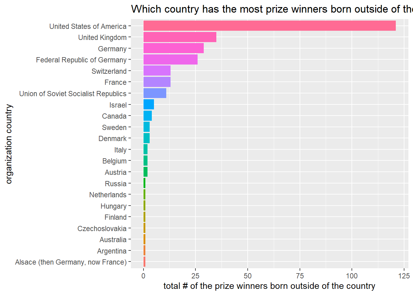
Immigration Nobel Prize Winners
winners %>%
  group_by(organization_country) %>%
  summarize(foreign_born_count = sum(birth_country != organization_country),
         total_count = n()) %>%
  mutate(foreign_born_ratio = foreign_born_count/total_count,
         organization_country = fct_reorder(organization_country, foreign_born_ratio)) %>%
  filter(foreign_born_ratio > 0) %>%
  ggplot(aes(foreign_born_ratio, organization_country, fill = organization_country)) +
  geom_col(show.legend = F) +
  scale_x_continuous(labels = percent) +
  labs(x = "percentage of foreign born winners",
       y = NULL,
title = "Percentage of Foreign Born Nobel Prize Winners") 
Gender including organizations
winners %>%
  mutate(gender = coalesce(gender, laureate_type)) %>%
  count(gender, category, sort = T) %>%
  drop_na() %>%
  complete(gender, category, fill = list(n = 0)) %>%
  ggplot(aes(gender, category, fill = n)) +
  geom_tile() +
  scale_fill_gradient2(
    high = "green",
    low = "red",
    mid = "white",
    midpoint = 100
  ) +
  scale_x_discrete(expand = c(0,0)) +
  scale_y_discrete(expand = c(0,0)) +
  labs(x = NULL,
       y = NULL,
       fill = "# of prize winners",
       title = "Total # of Nobel Prize Winners Across All Categories between Men, Women & Organization",
subtitle = "Organization was only awarded Peace Prize") 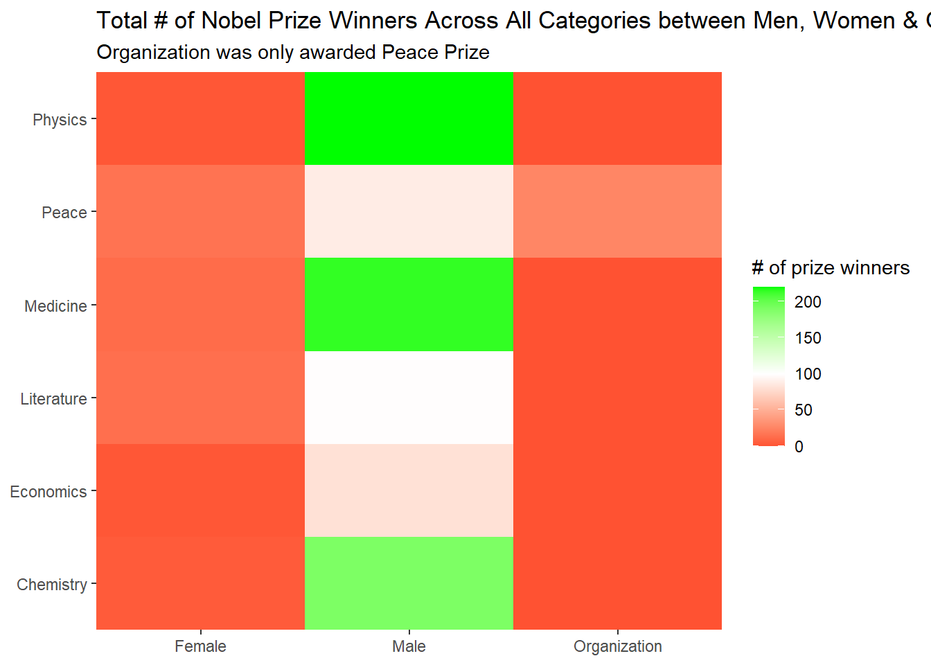
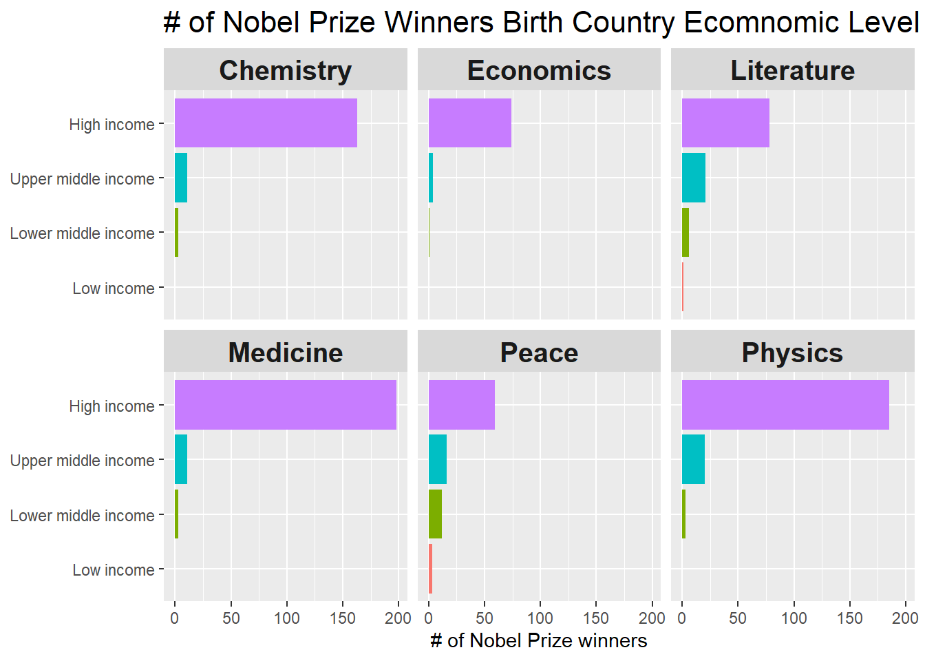
Birth Country’s economic situation
economy <- WDI(indicator = c("NY.GDP.PCAP.KD"), start = 2016, end = 2016, extra = T) %>%
  as_tibble()


winners %>%
  mutate(country_code = countrycode(birth_country, origin = 'country.name', destination = 'iso2c')) %>%
  inner_join(economy, by = c(country_code = "iso2c")) %>%
  count(category, income, sort = T) %>%
  mutate(income = fct_relevel(income, levels = c("Low income", "Lower middle income", "Upper middle income", "High income"))) %>%
  ggplot(aes(n, income, fill = income)) +
  geom_col(show.legend = F) +
  facet_wrap(~category) +
  theme(strip.text = element_text(size = 15, face = "bold"),
        plot.title = element_text(size = 16)) +
  labs(x = "# of Nobel Prize winners",
       y = NULL,
       title = "# of Nobel Prize Winners Birth Country Ecomnomic Level")