Plastic Waste (with Joins & WDI package)

Plastic products are ubiquitous in our everyday life, and they are always associated with waste and pollution to the global environment. In this blog post, we will analyze three releated dataset from TidyTuesday, shedding some light on how much plastic waste is produced in each country and how it is related to GDP and other key factors.

library(tidyverse)
library(WDI)
library(scales)
library(countrycode)

coast_vs_waste <- readr::read_csv("https://raw.githubusercontent.com/rfordatascience/tidytuesday/master/data/2019/2019-05-21/coastal-population-vs-mismanaged-plastic.csv") %>%
  janitor::clean_names()

mismanaged_vs_gdp <- readr::read_csv("https://raw.githubusercontent.com/rfordatascience/tidytuesday/master/data/2019/2019-05-21/per-capita-mismanaged-plastic-waste-vs-gdp-per-capita.csv")%>%
  janitor::clean_names()

waste_vs_gdp <- readr::read_csv("https://raw.githubusercontent.com/rfordatascience/tidytuesday/master/data/2019/2019-05-21/per-capita-plastic-waste-vs-gdp-per-capita.csv")%>%
  janitor::clean_names()

coast_vs_waste %>%
  summarise_all(~mean(is.na(.)))

## # A tibble: 1 x 6
##   entity  code  year mismanaged_plastic_w~ coastal_populati~ total_population_g~
##    <dbl> <dbl> <dbl>                 <dbl>             <dbl>               <dbl>
## 1      0     0     0                 0.991             0.991            0.000597

mismanaged_vs_gdp %>%
  summarise_all(~mean(is.na(.)))

## # A tibble: 1 x 6
##   entity   code  year per_capita_mismanage~ gdp_per_capita_ppp~ total_populatio~
##    <dbl>  <dbl> <dbl>                 <dbl>               <dbl>            <dbl>
## 1      0 0.0558     0                 0.992               0.711           0.0956

waste_vs_gdp %>%
  summarise_all(~mean(is.na(.)))

## # A tibble: 1 x 6
##   entity   code  year per_capita_plastic~ gdp_per_capita_ppp_c~ total_populatio~
##    <dbl>  <dbl> <dbl>               <dbl>                 <dbl>            <dbl>
## 1      0 0.0558     0               0.992                 0.711           0.0956

For some reason, some columns are dominated by the missing values.

coast_vs_waste %>%
  group_by(year) %>%
  summarize(total_pop = sum(total_population_gapminder)) %>% 
  ggplot(aes(year, total_pop)) +
  geom_line(size = 1) +
  scale_x_continuous(breaks = seq(1700, 2000, 50)) +
  labs(y = "global population",
       title = "Global Population from 1700 to 2000")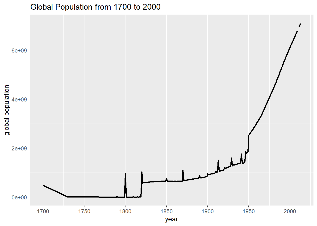

Join three tibbles together.

joined <- coast_vs_waste %>%
  filter(!is.na(mismanaged_plastic_waste_tonnes)) %>%
  inner_join(mismanaged_vs_gdp %>% select(-total_population_gapminder), by = c("entity", "year", "code")) %>%
  inner_join(waste_vs_gdp %>% select(-total_population_gapminder), by = c("entity", "year", "code")) %>% 
  select(-year) 

joined %>%
  ggplot(aes(mismanaged_plastic_waste_tonnes, coastal_population, color = code)) +
  geom_point() +
  scale_x_log10() +
  scale_y_log10() +
  geom_text(aes(label = code), check_overlap = T, vjust = 1, hjust = 1) +
  theme(legend.position = "none") +
  labs(x = "mismanaged plastic waste (tonnes)",
       y = "coastal population")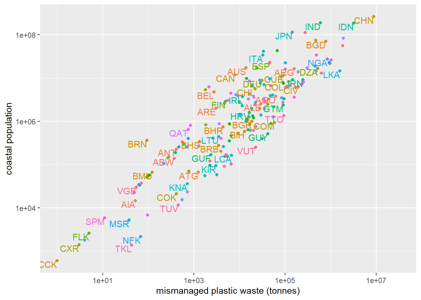 

There is a positive relationship between mismanged plastic waste and coastal population. This makes sense, as more poeple will produce more plastic, thus more plastic waste.

joined %>%
  ggplot(aes(mismanaged_plastic_waste_tonnes, gdp_per_capita_ppp_constant_2011_international_rate, color = code)) +
  geom_point() +
  scale_x_log10() +
  scale_y_log10(labels = dollar) +
  geom_hline(yintercept = 10000, color = "red") +
  geom_text(aes(label = code), check_overlap = T, vjust = 1, hjust = 1) +
  theme(legend.position = "none") +
  labs(x = "mismanaged plastic waste (tonnes)",
       y = "GDP per capita")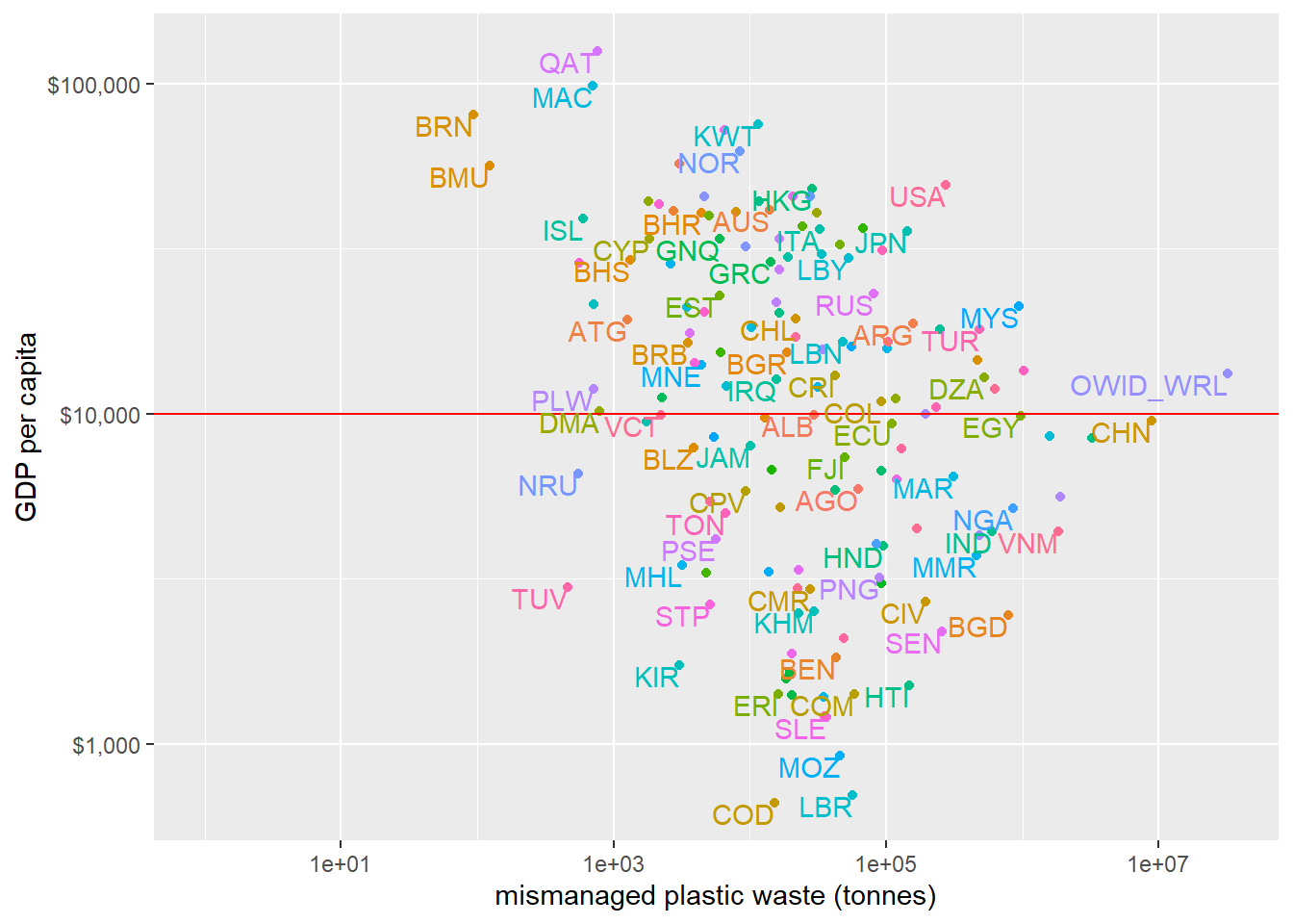 

joined %>%
  ggplot(aes(per_capita_mismanaged_plastic_waste_kilograms_per_person_per_day, gdp_per_capita_ppp_constant_2011_international_rate, color = code)) +
  geom_point() +
  scale_x_log10() +
  scale_y_log10(labels = dollar) +
  geom_hline(yintercept = 10000, color = "red") +
  geom_text(aes(label = entity), check_overlap = T, vjust = 1, hjust = 1) +
  theme(legend.position = "none") +
  labs(x = "mismanaged plastic waste per person per day",
       y = "GDP per capita")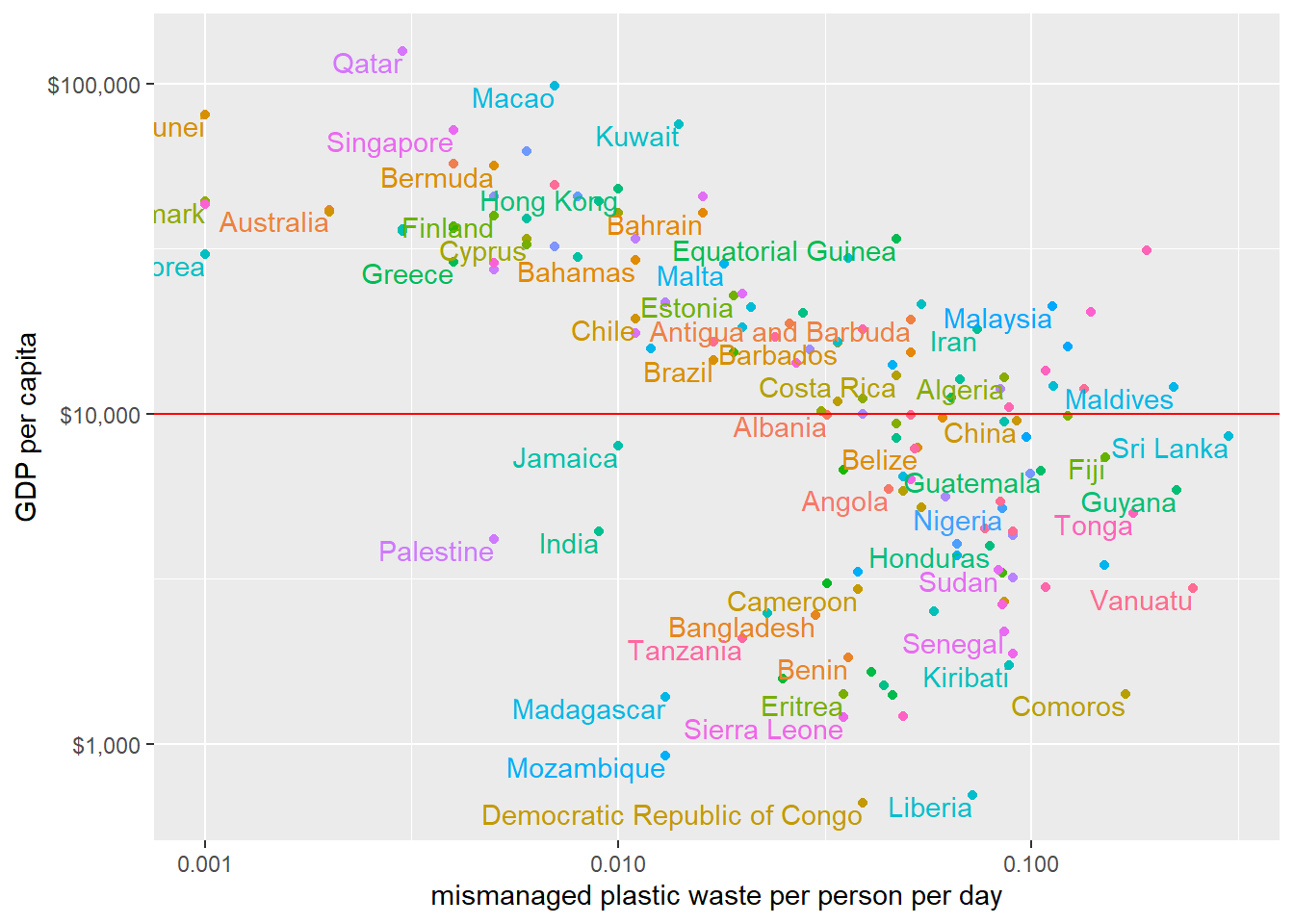 

The plot above shows there is something wrong about the data entry, as GDP per capita for many countries above the red horizontal line (> $10,000) do not reflect the fact.

carbon_emission <- joined %>%
  inner_join(
    WDI(indicator = "EN.ATM.CO2E.PC", start = 2010, end = 2010) %>% 
      rename("carbon_emission" = "EN.ATM.CO2E.PC") %>%
      mutate(code = countrycode(country, origin = 'country.name', destination = 'iso3c')), by = "code"
  )

carbon_emission %>% 
  ggplot(aes(per_capita_mismanaged_plastic_waste_kilograms_per_person_per_day, carbon_emission, color = code)) +
  geom_point() +
  scale_y_log10() +
  scale_x_log10() +
  geom_text(aes(label = code), check_overlap = T, vjust = 1, hjust = 1) +
  theme(legend.position = "none") +
  labs(x = "mismanaged plastic waste (kg per person per day)",
       y = "carbon emission")