Wine Rating Data Visualization and Lasso Model on Word Prediction
Wed, Nov 3, 2021
4-minute read
This blog post will analyze an interesting wine dataset from TidyTuesday. We will visualize the data and use a LASSO model to use words presented in the wine description to make prediction for wine rating.
library(tidyverse)
library(scales)
library(patchwork)
library(broom)
library(tidytext)
library(geofacet)
library(glmnet)
theme_set(theme_bw())
wine <- read_csv("https://raw.githubusercontent.com/rfordatascience/tidytuesday/master/data/2019/2019-05-28/winemag-data-130k-v2.csv") %>%
filter(!is.na(price)) %>%
select(-X1)
wine## # A tibble: 120,975 x 13
## country description designation points price province region_1 region_2
## <chr> <chr> <chr> <dbl> <dbl> <chr> <chr> <chr>
## 1 Portugal This is ripe ~ Avidagos 87 15 Douro <NA> <NA>
## 2 US Tart and snap~ <NA> 87 14 Oregon Willame~ Willame~
## 3 US Pineapple rin~ Reserve Lat~ 87 13 Michigan Lake Mi~ <NA>
## 4 US Much like the~ Vintner's R~ 87 65 Oregon Willame~ Willame~
## 5 Spain Blackberry an~ Ars In Vitro 87 15 Northern~ Navarra <NA>
## 6 Italy Here's a brig~ Belsito 87 16 Sicily &~ Vittoria <NA>
## 7 France This dry and ~ <NA> 87 24 Alsace Alsace <NA>
## 8 Germany Savory dried ~ Shine 87 12 Rheinhes~ <NA> <NA>
## 9 France This has grea~ Les Natures 87 27 Alsace Alsace <NA>
## 10 US Soft, supple ~ Mountain Cu~ 87 19 Californ~ Napa Va~ Napa
## # ... with 120,965 more rows, and 5 more variables: taster_name <chr>,
## # taster_twitter_handle <chr>, title <chr>, variety <chr>, winery <chr>Rated Points & Wine Price
p1 <- wine %>%
  mutate(country = fct_lump(country, n = 10)) %>%
  filter(country != "Other") %>%
  ggplot(aes(points, country, fill = country)) +
  geom_violin(show.legend = F) +
  labs(y = NULL,
       title = "Top 10 Wine Produced Countries with Rated Points") +
  theme(
    axis.title = element_text(size = 15),
    axis.text = element_text(size = 13),
    plot.title = element_text(size = 18)
  )


p2 <- wine %>%
  mutate(country = fct_lump(country, n = 10)) %>%
  filter(country != "Other") %>%
  ggplot(aes(price, country, fill = country)) +
  geom_violin(show.legend = F) +
  labs(y = NULL,
       x = "price",
       title = "Top 10 Wine Produced Countries with Price") +
  theme(
    axis.title = element_text(size = 15),
    axis.text = element_text(size = 13),
    plot.title = element_text(size = 18)
  ) +
  scale_x_log10(labels = dollar)

p1 + p2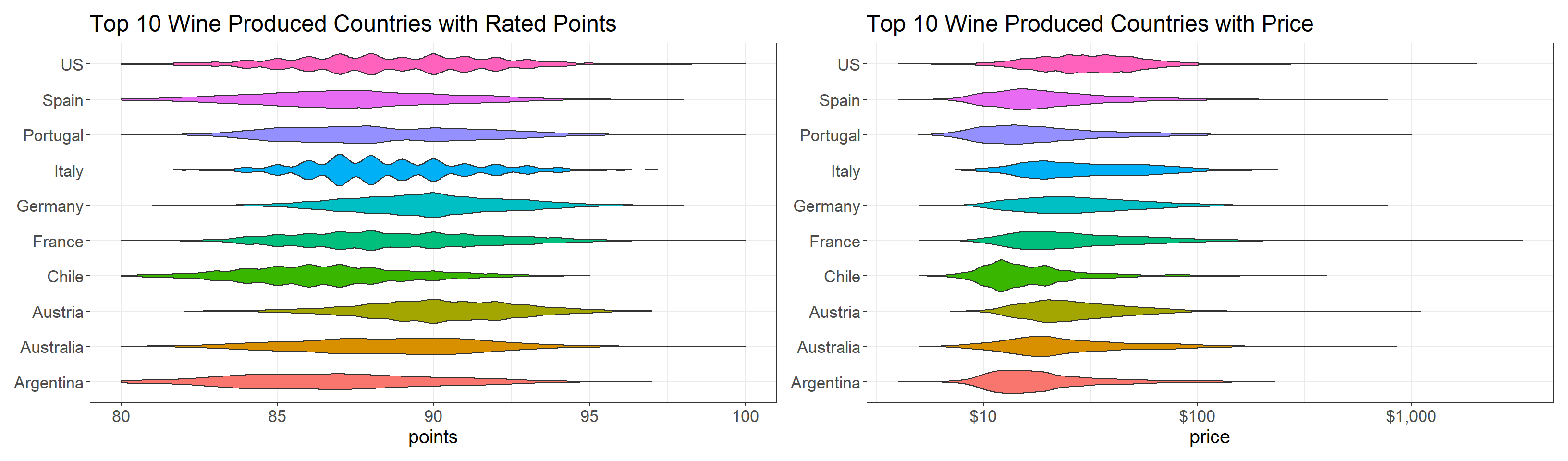
Grape types
wine %>%
  count(variety, sort = T) %>%
  head(20) %>%
  mutate(variety = fct_reorder(variety, n)) %>%
  ggplot(aes(n, variety, fill = variety)) +
  geom_col(show.legend = F) +
  labs(x = NULL,
       y = NULL,
title = "Top 20 Grape Variety Distribution") 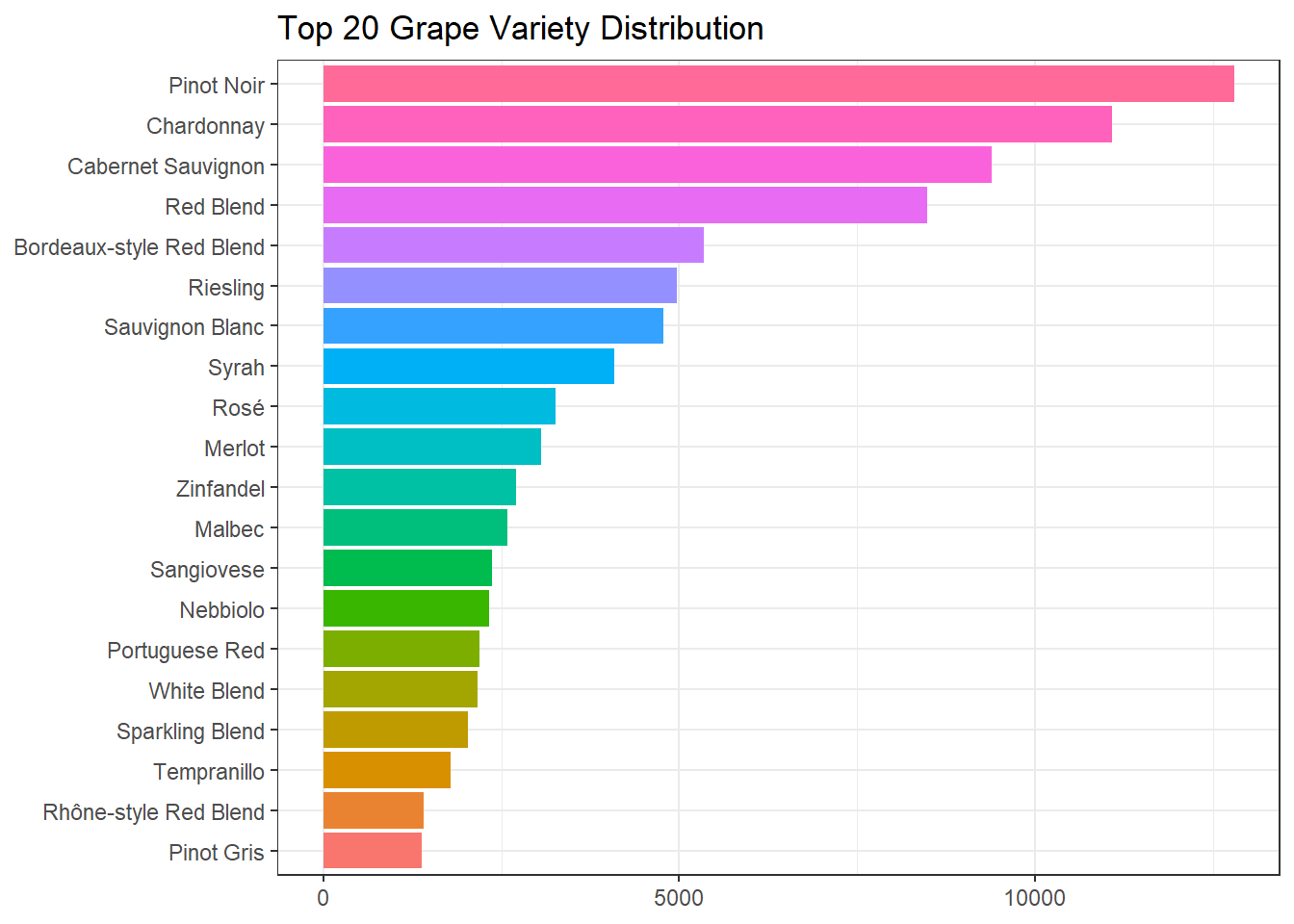
wine %>%
  mutate(taster_name = fct_lump(taster_name, n = 20),
         taster_name = fct_reorder(taster_name, points, median, na.rm = T)) %>%
  filter(!is.na(taster_name)) %>%
  ggplot(aes(points, taster_name, fill = taster_name)) +
  geom_boxplot(show.legend = F) +
  labs(y = "taster",
title = "The 20 Most Popular Tasters and Their Wine Ratings") 
wine %>%
  mutate(winery = fct_lump(winery, n = 30)) %>%
  nest(-winery) %>%
  filter(winery != "Other") %>%
  mutate(model = map(data, ~ t.test(.$points)),
         tidied = map(model, tidy)) %>%
  unnest(tidied) %>%
  mutate(winery = fct_reorder(winery, estimate)) %>%
  ggplot(aes(estimate, winery)) +
  geom_point() +
  geom_errorbarh(aes(xmin = conf.low, xmax = conf.high)) +
  labs(x = "point estimate",
       title = "Top 30 Popular Winery Point Estimate")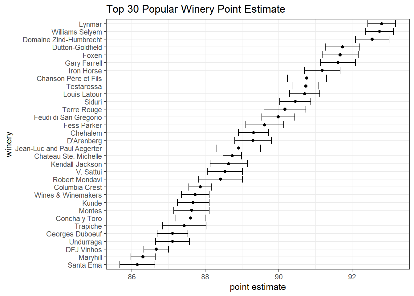
Wine description analysis
wine %>%
  select(description, country) %>%
  unnest_tokens(word, description) %>%
  anti_join(stop_words) %>%
  count(country, word, sort = T) %>%
  head(100) %>%
  mutate(word = fct_reorder(word, n, sum)) %>%
  ggplot(aes(n, word, fill = country)) +
  geom_col() +
  labs(x = "word count",
       y = "wine description word",
       title = "The Most Frequent Wine Description Words")
## Joining, by = "word"
US wine
us_wine <- wine %>%
  filter(country == "US") %>%
  rename(state = "province")

agg_data <- us_wine %>%
  group_by(state) %>%
  summarize_at(vars(points, price), mean, na.rm = T) %>%
  ungroup()


joined <- map_data("state") %>%
  left_join(
    agg_data %>%
      mutate(state = str_to_lower(state)),
    by = c("region" = "state")
  )

p3 <- joined %>%
  ggplot(aes(long, lat, group = group, fill = points)) +
  geom_polygon() +
  coord_map() +
  theme_void() +
  scale_fill_gradient2(high = "green",
                       low = "red",
                       mid = "pink",
                       midpoint =  86) +
  labs(fill = "wine rating",
       title = "Average Wine Rating in the U.S.")

p4 <- joined %>%
  ggplot(aes(long, lat, group = group, fill = price)) +
  geom_polygon() +
  coord_map() +
  theme_void() +
  scale_fill_gradient2(high = "green",
                       low = "red",
                       mid = "pink",
                       midpoint =  25) +
  labs(fill = "wine pricing",
       title = "Average Wine Pricing in the U.S.")

p3 / p4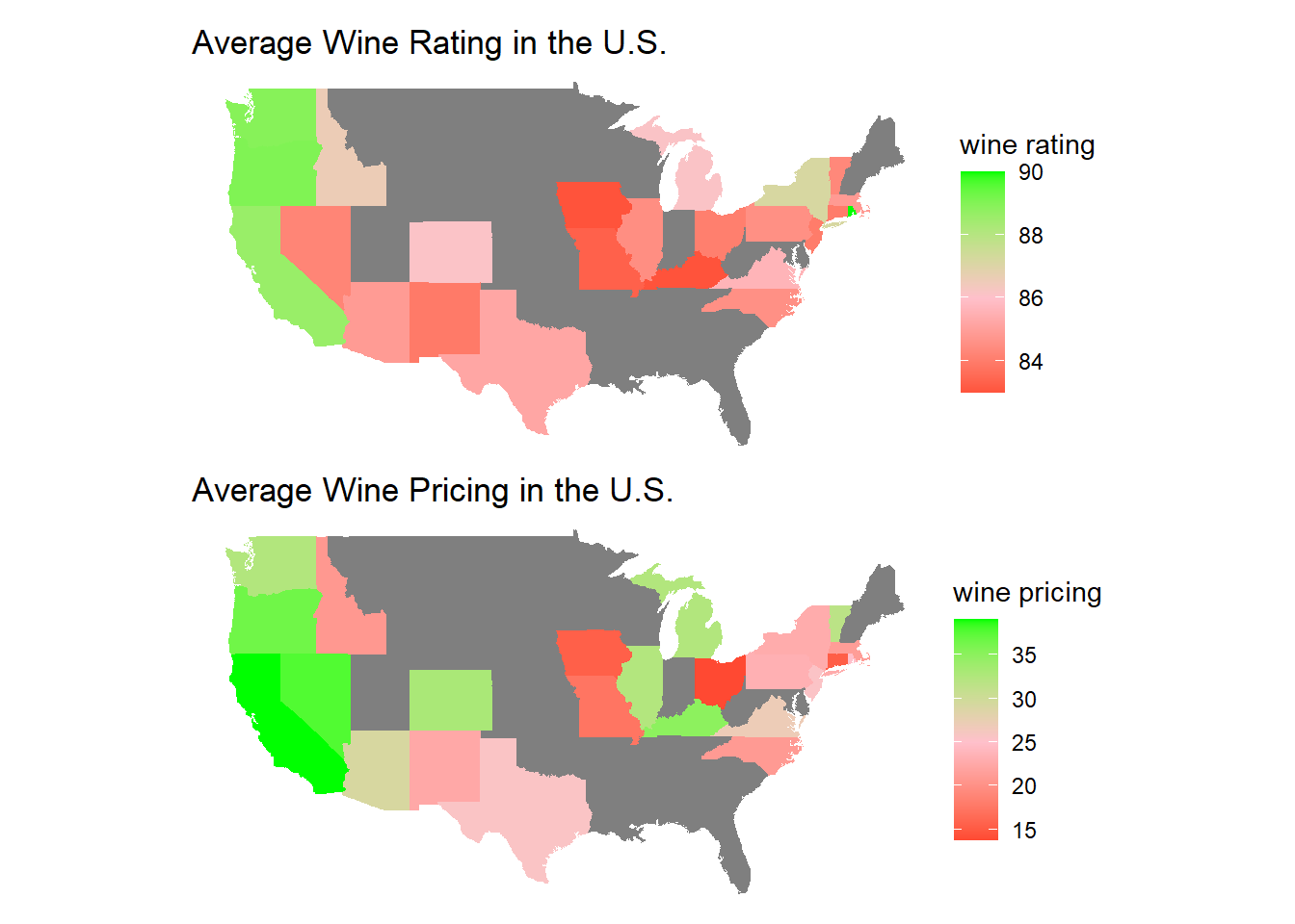
Ohio has not so good wine compared to other states, but the wine price is relatively cheaper as well. There are always pros and cons, depending on how you look at it.
Lasso model
This chunk of code is highly inspired by David Robinson’s code on using Lasso model on word prediction with cast_sparse().
desc_matrix <- wine %>%
  mutate(wine_id = row_number()) %>%
  unnest_tokens(word, description) %>%
  anti_join(stop_words) %>%
  distinct(wine_id, word) %>%
  add_count(word) %>%
  filter(n > 100) %>%
  cast_sparse(wine_id, word)

# Lining up points with wine_id

wine_id <- as.integer(rownames(desc_matrix))

points <- wine$points[wine_id]

wine_word_matrix_extra <- cbind(desc_matrix, log_price = log2(wine$price[wine_id]))

cv_glmnet_model <- cv.glmnet(wine_word_matrix_extra, points)

plot(cv_glmnet_model)
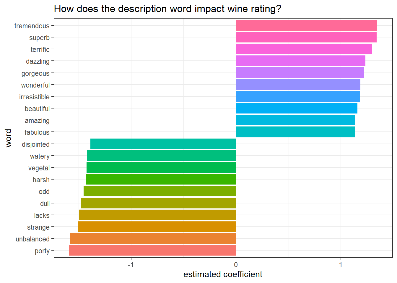
cv_glmnet_model$glmnet.fit %>%
  tidy() %>%
  filter(!str_detect(term, "(Intercept)|log_price"),
         lambda == cv_glmnet_model$lambda.1se) %>%
  select(word = term, coefficient = estimate) %>%
  mutate(direction = if_else(coefficient < 0, "negative", "positive")) %>%
  group_by(direction) %>%
  slice_max(abs(coefficient), n = 10) %>%
  ungroup() %>%
  mutate(word = fct_reorder(word, coefficient)) %>%
  ggplot(aes(coefficient, word, fill = word)) +
  geom_col(show.legend = F) +
  labs(x = "estimated coefficient",
       y = "word",
       title = "How does the description word impact wine rating?")