Web Scraping & Visualization on American Statistical Association Fellows

I came across the wikipedia page on ASA Fellows. Since my Ph.D. advisor is ASA fellow, it is interesting to web scrape the page by using the R package rvest and then analyze the data after obatining it.

Load the packages!

library(tidyverse)
library(rvest)

The webpage only contains the full name of each fellow and year. In order to get first, middle and last name, I need to do some data wrangling. This turns out to be a bit harder than I thought, as some fellows (for example, the Chinese) do not have middle name.

Some useful functions are used here (na_if() and fill()).

asa <- read_html("https://en.wikipedia.org/wiki/List_of_fellows_of_the_American_Statistical_Association") %>%
  html_nodes(".div-col li , h3 .mw-headline") %>%
  html_text() %>%
  as_tibble() %>%
  mutate(year = if_else(str_detect(value, "[:digit:]"), value, "Missing")) %>%
  mutate(year = na_if(year, "Missing")) %>%
  fill(year) %>%
  mutate(year = as.numeric(year)) %>%
  filter(!str_detect(value, "[:digit:]")) %>%
  rename(name = "value") %>%
  separate(name, into = c("first_name", "middle_last_name"), sep = " ", extra = "merge", remove = F) %>%
  separate(middle_last_name, into = c("middle_name", "last_name"), sep = " ", fill = "left")

asa

## # A tibble: 3,024 x 5
##    name                    first_name middle_name last_name  year
##    <chr>                   <chr>      <chr>       <chr>     <dbl>
##  1 John Lee Coulter        John       Lee         Coulter    1914
##  2 Miles Menander Dawson   Miles      Menander    Dawson     1914
##  3 Frank H. Dixon          Frank      H.          Dixon      1914
##  4 David Parks Fackler     David      Parks       Fackler    1914
##  5 Henry Walcott Farnam    Henry      Walcott     Farnam     1914
##  6 Charles Ferris Gettemy  Charles    Ferris      Gettemy    1914
##  7 Franklin Henry Giddings Franklin   Henry       Giddings   1914
##  8 Henry J. Harris         Henry      J.          Harris     1914
##  9 Edward M. Hartwell      Edward     M.          Hartwell   1914
## 10 Joseph A. Hill          Joseph     A.          Hill       1914
## # ... with 3,014 more rows

asa %>%
  count(year) %>%
  ggplot(aes(year, n)) +
  geom_line() +
  geom_point() +
  scale_x_continuous(breaks = seq(1914, 2021, by = 15)) +
  labs(y = "# of ASA Fellows awarded",
       title = "How many American Statistical Association Fellows are awarded each year?")

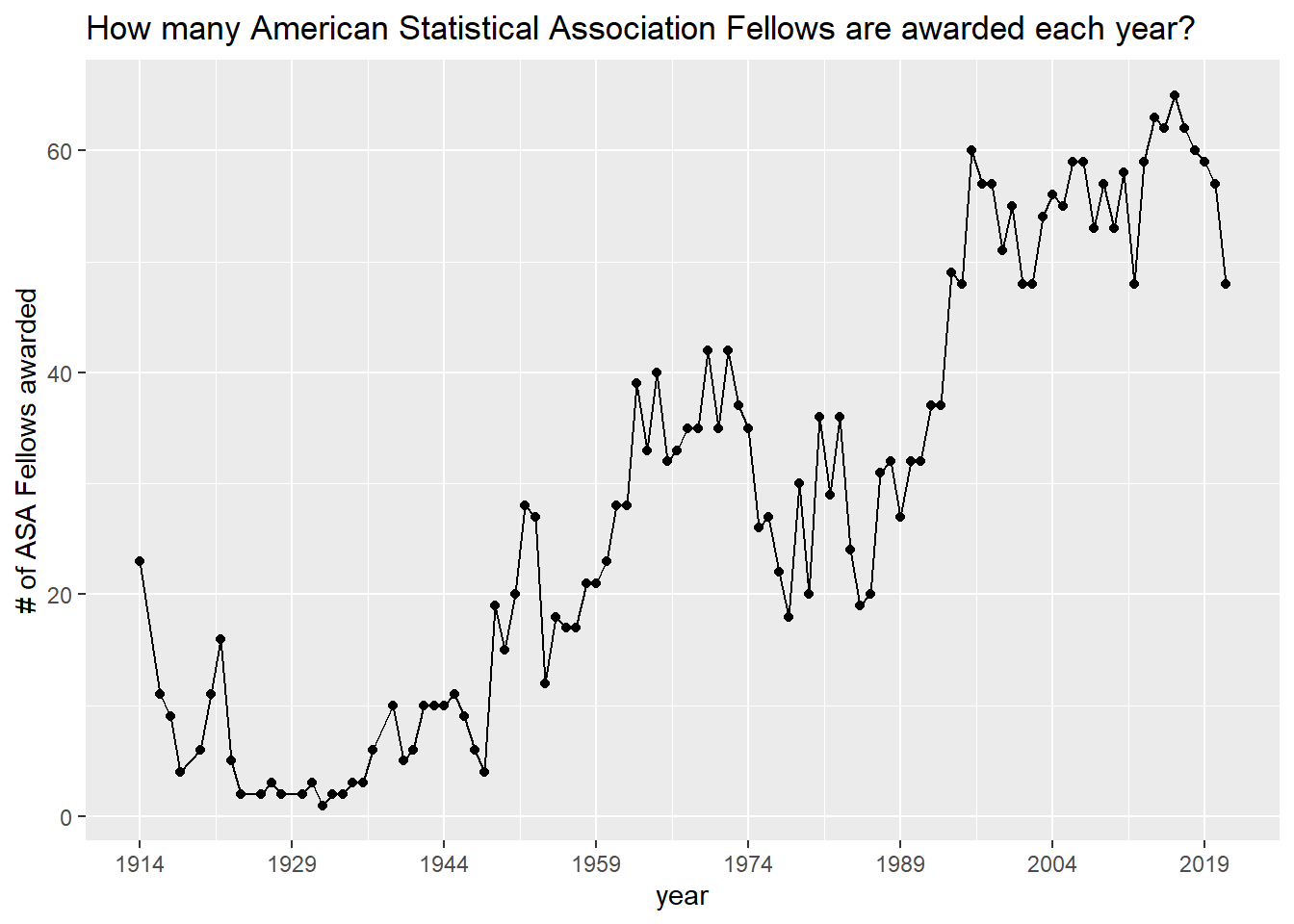
There is a generally upward trend for the number of fellows awarded each year.

asa %>%
  mutate(decade = 10 * floor(year / 10)) %>%
  count(decade) %>%
  filter(decade != 2020) %>%
  ggplot(aes(decade, n, fill = as.factor(decade))) +
  geom_col(show.legend = F) +
  scale_x_continuous(breaks = seq(1910, 2020, 10)) +
  labs(y = "# of ASA Fellows awarded",
       title = "How many American Statistical Association Fellows are awarded each decade?")

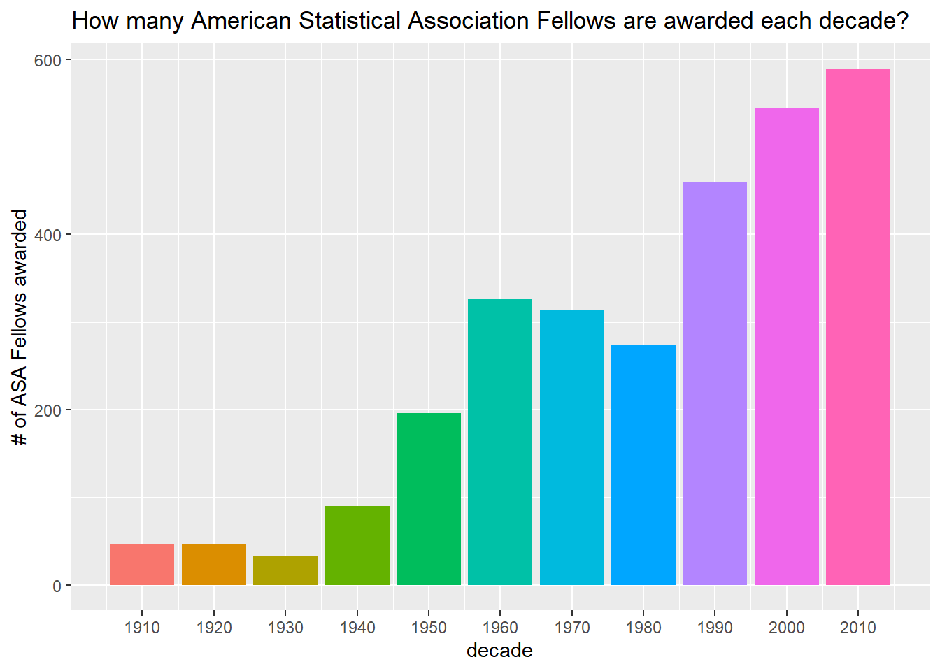
Indeed, 2010-2019 is the largest decade in terms of # of ASA fellows.

asa %>%
  mutate(last_name = fct_lump(last_name, 10)) %>%
  count(last_name) %>%
  filter(last_name != "Other") %>%
  mutate(last_name = fct_reorder(last_name, n)) %>%
  ggplot(aes(n, last_name, fill = last_name)) +
  geom_col(show.legend = F) +
  labs(x = "# of ASA Fellows awarded",
       y = "last name",
       title = "Top 10 family names awarded ASA Fellows") 

asa %>%
  mutate(first_name = fct_lump(first_name, 10)) %>%
  count(first_name) %>%
  filter(first_name != "Other") %>%
  mutate(first_name = fct_reorder(first_name, n)) %>%
  ggplot(aes(n, first_name, fill = first_name)) +
  geom_col(show.legend = F) +
  labs(x = "# of ASA Fellows awarded",
       y = "first name",
       title = "Top 10 first names awarded ASA Fellows")