Women World Cup Visualization & Prediction

Join wwc_outcomes and codes together

wwc_joined <- wwc_outcomes %>%
  left_join(codes, by = "team") %>%
  mutate(round = fct_relevel(round, "Group", "Quarter Final", "Round of 16", "Semi Final", "Third Place Playoff", "Final"))

Total wins

wwc_joined %>%
  group_by(country) %>%
  summarize(total_wins = sum(win_status == "Won")) %>%
  ungroup() %>%
  filter(total_wins > 0) %>%
  mutate(country = fct_reorder(country, total_wins)) %>%
  ggplot(aes(total_wins, country, fill = country)) +
  geom_col(show.legend = F) +
  labs(x = "total # of wins",
       y = NULL,
       title = "Total Wins from 1991 to 2019")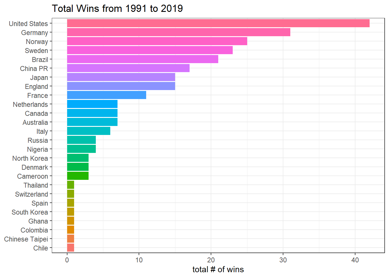 

Champs

wwc_joined %>%
  filter(round == "Final") %>%
  group_by(country) %>%
  summarize(`number of champs` = sum(win_status == "Won"),
            `number of finals` = n()) %>%
  ungroup() %>%
  pivot_longer(-country) %>%
  ggplot(aes(value, country, fill = name)) +
  geom_col(position = "dodge") +
  labs(x = NULL,
       y = NULL,
       fill = NULL,
       title = "# of Times When Playing into Final & Winning the Champs")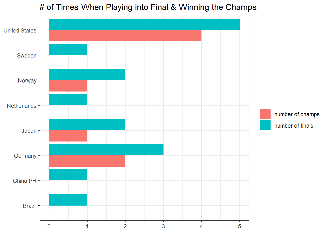

Third Place Playoff

wwc_joined %>%
  filter(round == "Third Place Playoff") %>%
  group_by(country) %>%
  summarize(`the third` = sum(win_status == "Won"),
            `number of third place playoff` = n()) %>%
  ungroup() %>%
  pivot_longer(-country) %>%
  ggplot(aes(value, country, fill = name)) +
  geom_col(position = "dodge") +
  labs(x = NULL,
       y = NULL,
       fill = NULL,
       title = "# of Times When Getting the Third Position")

First four

wwc_joined %>%
  filter(round %in% c("Third Place Playoff", "Final")) %>%
  mutate(medal = case_when(
    round == "Final" & win_status == "Won" ~ "Gold",
    round == "Final" & win_status == "Lost" ~ "Silver",
    round == "Third Place Playoff" & win_status == "Won" ~ "Broze",
    round == "Third Place Playoff" & win_status == "Lost" ~ "4th",
  )) %>%
  mutate(medal = fct_relevel(medal, "Gold", "Silver", "Broze", "4th")) %>%
  ggplot(aes(year, medal, color = country)) +
  geom_point() +
  geom_text(aes(label = country), hjust = 0, vjust = 1, check_overlap = T) +
  theme(legend.position = "none",
        panel.grid = element_blank()) +
  scale_x_continuous(breaks = unique(wwc_joined$year)) +
  labs(x = NULL,
       y = NULL,
       title = "The First Four Positions of Women's World Cup")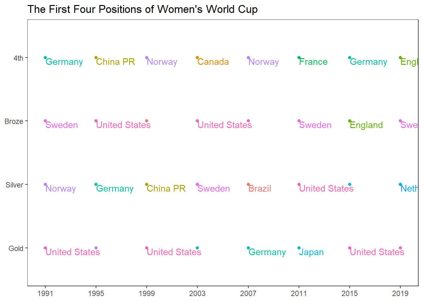 

Predicitons

This little section is inspired by David Robinson’s code. The link is here.

outcomes <- wwc_joined %>%
  group_by(year, yearly_game_id) %>%
  mutate(rev_score = rev(score),
         score_diff = score - rev_score) %>%
  ungroup()

wwc_group_score <- outcomes %>%
  filter(round == "Group") %>%
  group_by(year, team) %>%
  summarize(avg_group_score = mean(score, na.rm = T),
            avg_score_diff = mean(score_diff, na.rm = T))

## `summarise()` has grouped output by 'year'. You can override using the `.groups` argument.

outcomes %>%
  inner_join(wwc_group_score, by = c("year", "team")) %>%
  filter(round == "Final") %>%
  mutate(year = paste(year, "Final")) %>%
  ggplot(aes(country, avg_group_score, fill = win_status)) +
  geom_col() +
  facet_wrap(~year, scales = "free_x") +
  theme(legend.position = c(0.8, 0.15)) +
  labs(x = NULL,
       y = "mean score in the Group round",
       fill = NULL,
       title = "Can the mean score in the Group round predict if a team won in Final?",
       subtitle = "It seems like it can! (except 2011)")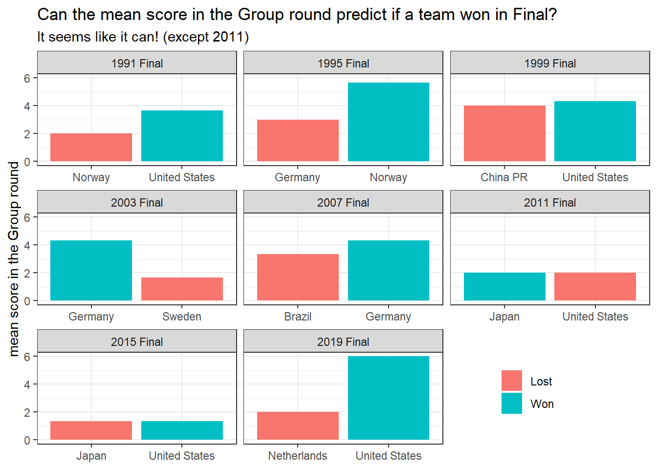

Working on squads

It is interesting to see which position would score most.

squads %>%
  group_by(pos) %>%
  summarize(avg_goals = mean(goals, na.rm = T))

## # A tibble: 4 x 2
##   pos   avg_goals
##   <chr>     <dbl>
## 1 DF         3.07
## 2 FW        16.2 
## 3 GK         0   
## 4 MF         7.54

squads %>%
  filter(goals > 0) %>%
  mutate(pos = fct_reorder(pos, goals, median, na.rm = T)) %>%
  ggplot(aes(goals, pos, fill = pos)) +
  geom_boxplot(show.legend = F) +
  scale_x_log10() +
  labs(x = "# of goals",
       y = "position") 

Forward will get scores more often than other positions on the filed.

squads %>%
  group_by(pos) %>%
  summarize(sum = sum(goals, na.rm = T)) %>%
  arrange(desc(sum)) %>%
  pull(pos)

## [1] "FW" "MF" "DF" "GK"

squads %>%
  mutate(pos = fct_relevel(pos, "FW", "MF", "DF", "GK")) %>%
  ggplot(aes(age, goals, color = pos)) +
  geom_point() +
  geom_smooth() +
  facet_wrap(~pos) +
  theme(legend.position = "none") +
  labs(title = "# of Goals V.S. Age Faceted by Position with Loess Curve")

## `geom_smooth()` using method = 'loess' and formula 'y ~ x'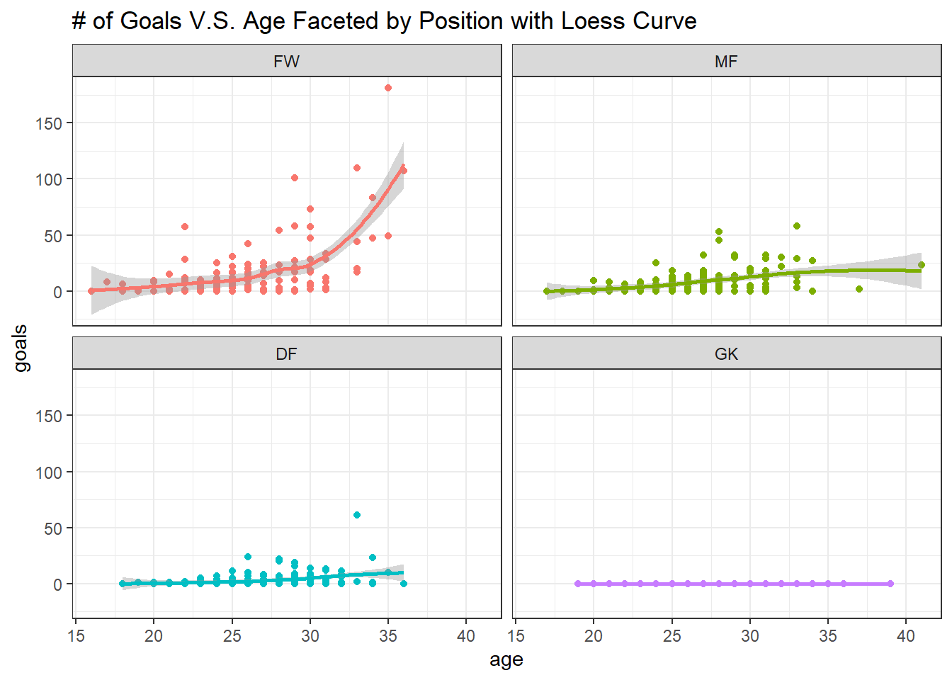

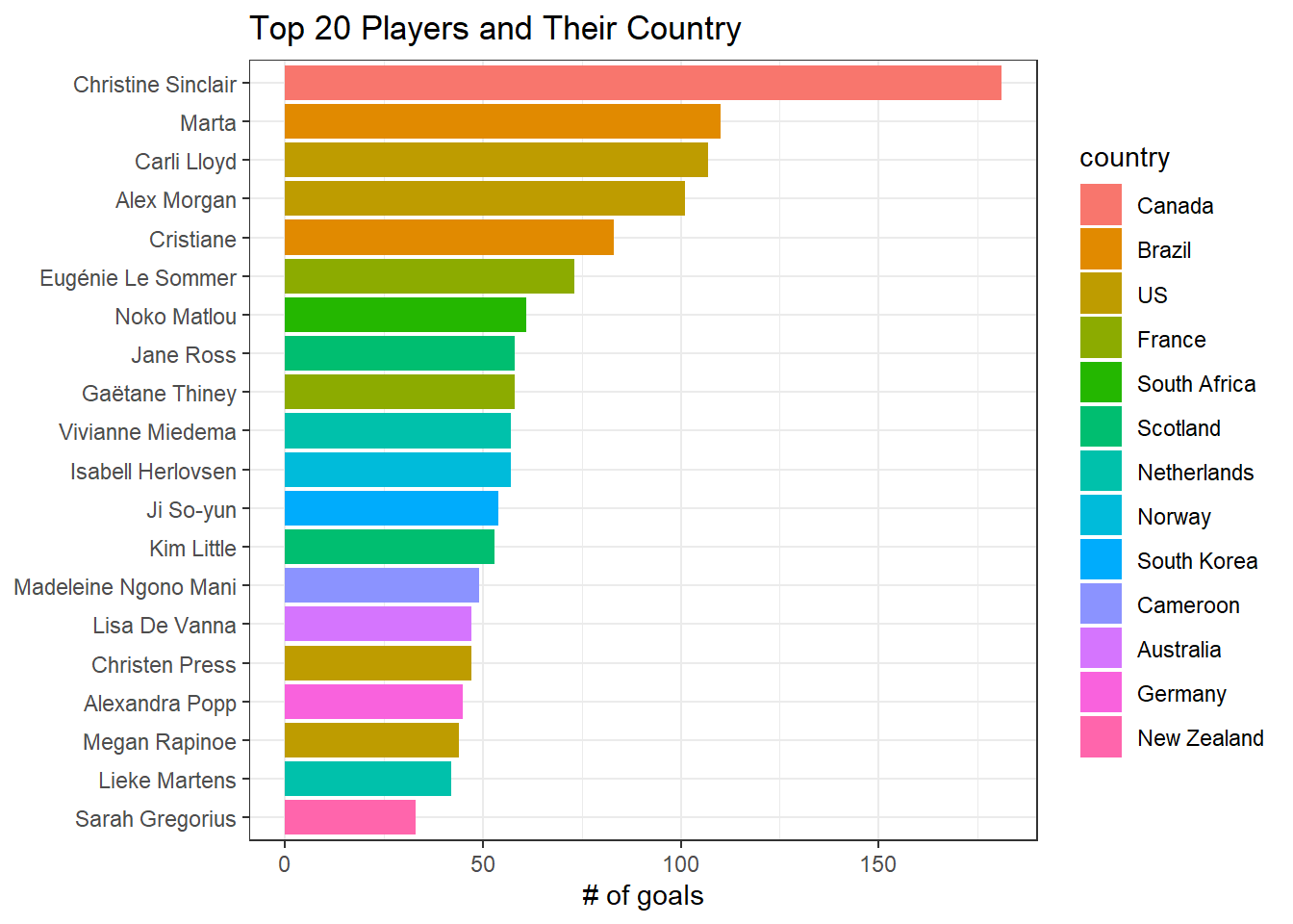
Top 20 Players

squads %>%
  arrange(desc(goals)) %>%
  head(20) %>%
  mutate(player = fct_reorder(player, goals),
         country = fct_reorder(country, -goals, min)) %>%
  ggplot(aes(goals, player, fill = country)) +
  geom_col() +
  labs(x = "# of goals",
       y = NULL,
       title = "Top 20 Players and Their Country")