Pizza Restaurant Data Visualization

Fri, Nov 26, 2021 3-minute read

This blog post analyzes a number of datasets related to Pizza, and they are from TidyTuesday Data Science Project.

library(tidyverse)
library(scales)
library(tidytext)
library(broom)

Using as.POSIXct() to transfrom non-sense time object into actual date.

pizza_jared <- read_csv("https://raw.githubusercontent.com/rfordatascience/tidytuesday/master/data/2019/2019-10-01/pizza_jared.csv") %>%
  filter(answer != "Fair") %>%
  mutate(answer = factor(answer, levels = c("Never Again", "Poor", "Average", "Good", "Excellent")),
         time = as.Date(as.POSIXct(time, origin = "1970-01-01")))

pizza_barstool <- read_csv("https://raw.githubusercontent.com/rfordatascience/tidytuesday/master/data/2019/2019-10-01/pizza_barstool.csv")
pizza_datafiniti <- read_csv("https://raw.githubusercontent.com/rfordatascience/tidytuesday/master/data/2019/2019-10-01/pizza_datafiniti.csv")

Pizza Restaurant Likert Scale

pizza_jared %>%
  group_by(place, answer) %>%
  summarize(votes = sum(votes),
            total_votes = sum(total_votes)) %>%
  mutate(percent = votes/total_votes) %>%
  ungroup() %>%
  ggplot(aes(answer, place, fill = percent)) +
  geom_tile() +
  scale_fill_gradient2(labels = percent,
                       low = "white",
                       high = "green",
                       mid = "pink",
                       midpoint = 0.5) +
  labs(x = "likert scale",
       y = NULL,
       fill = NULL,
       title = "Pizza Restaurant Likert Scale") +
  scale_x_discrete(expand = c(0,0))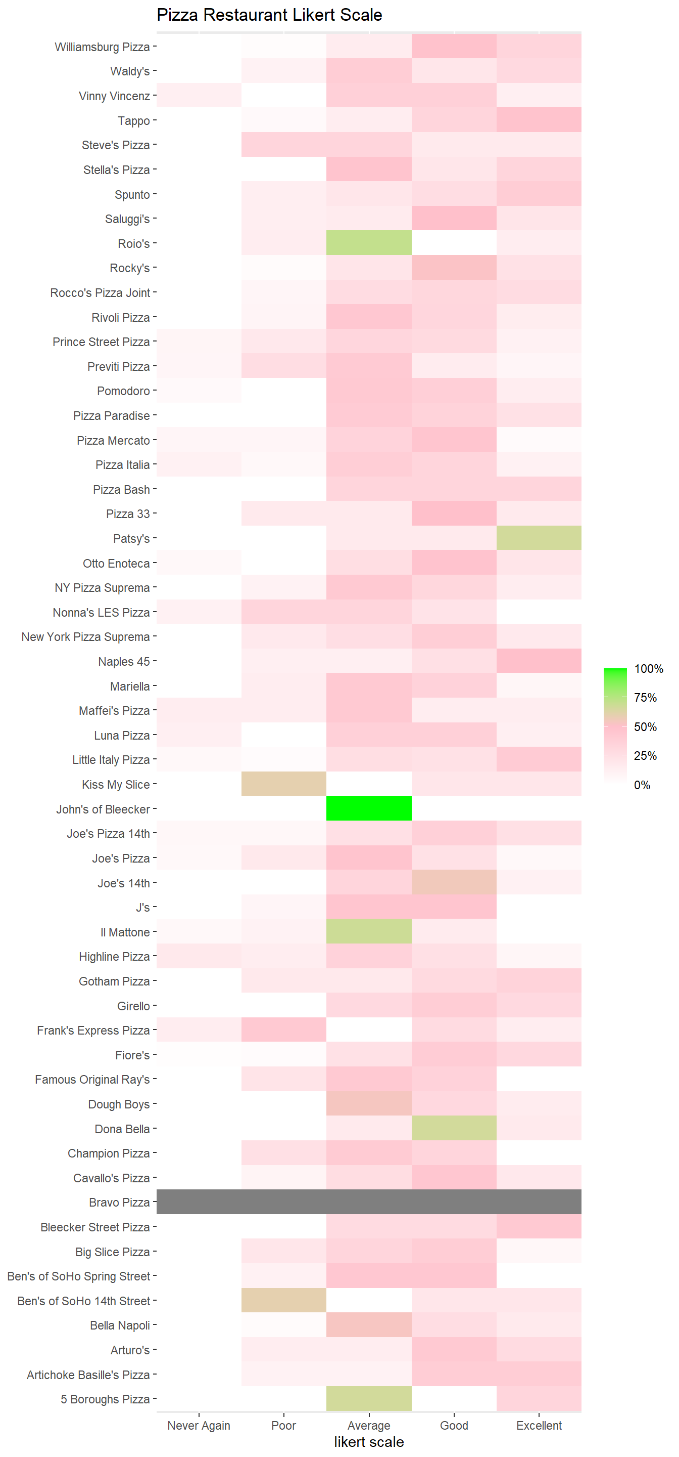

It seems like Patsy’s has the highest rating for being Excellent.

Now combining pizza_barstool and pizza_datafiniti together by using left_join().

pizza_combined <- pizza_barstool %>%
  left_join(pizza_datafiniti %>% select(name, price_range_min, price_range_max), by = "name") %>%
  distinct(name, .keep_all = T)

The ratings from cities with most of pizza restaurants

pizza_score <- pizza_combined %>%
  mutate(city = fct_lump(city, n = 5)) %>%
  filter(city != "Other") %>%
  select(name, city, price_level, contains("average_score")) %>%
  rename("restaurant" = "name") %>%
  pivot_longer(-c(restaurant, city, price_level)) %>% 
  mutate(name = str_remove(name, "review_stats_"),
         name = str_replace_all(name, "_"," ")) 

pizza_score %>%
  mutate(city = reorder_within(city, value, name, median)) %>%
  ggplot(aes(value, city, fill = city)) +
  geom_boxplot(show.legend = F) +
  scale_y_reordered() +
  facet_wrap(~name, scales = "free_y") +
  labs(x = "score",
       y = NULL,
       title = "Which city has the best Pizza rating?")

T-test prediction

pizza_score %>%
  nest(-c(city, name)) %>%
  mutate(model = map(data, ~ t.test(.$value)),
         tidied = map(model, tidy)) %>%
  unnest(tidied) %>%
  mutate(city = reorder_within(city, estimate, name)) %>%
  ggplot(aes(estimate, city)) +
  geom_point() +
  geom_errorbarh(aes(xmin = conf.low,
                     xmax = conf.high)) +
  facet_wrap(~name, scales = "free_y") +
  scale_y_reordered() +
  labs(x = "t-test score estimate",
       y = NULL,
       title = "Score estimates for each city")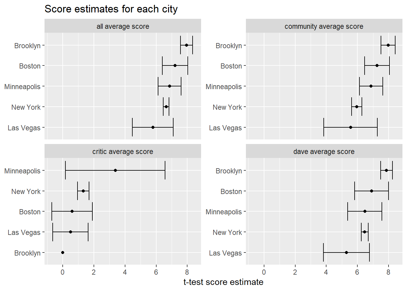

Making a map

pizza_combined %>%
  ggplot(aes(longitude, latitude, color = provider_rating)) +
  geom_point(size = 2) +
  borders("state") +
  theme_void() +
  coord_map() +
  labs(color = "provider rating",
       title = "Where are these pizza restaurants?")

## Warning: Removed 2 rows containing missing values (geom_point).

Price level and review rating

pizza_score %>%
  filter(price_level > 0) %>%
  mutate(price_level = as.character(price_level),
         price_level = fct_recode(price_level, "$" = "1", "$$" = "2", "$$$" = "3")) %>%
  ggplot(aes(value, fill = price_level)) +
  geom_histogram(alpha = 0.8, position = "dodge") +
  facet_wrap(~name) +
  labs(x = "rating",
       fill = "price level",
       title = "The distribution of scores among pizza restaurants from various price levels")

## `stat_bin()` using `bins = 30`. Pick better value with `binwidth`.

It looks like how much money spends on restaurant does not necessarily mean how high the rating it gets.