The Office Rating Data Visualization & Lasso Models
This blog post analyzes the TV Show The Office. This dataset comes from TidyTuesday, the data science online community.
library(tidyverse)
library(schrute)
library(lubridate)
library(tidytext)
library(Matrix)
library(glmnet)
library(broom)
theme_set(theme_bw())
office <- read_csv("https://raw.githubusercontent.com/rfordatascience/tidytuesday/master/data/2020/2020-03-17/office_ratings.csv")
office## # A tibble: 188 x 6
## season episode title imdb_rating total_votes air_date
## <dbl> <dbl> <chr> <dbl> <dbl> <date>
## 1 1 1 Pilot 7.6 3706 2005-03-24
## 2 1 2 Diversity Day 8.3 3566 2005-03-29
## 3 1 3 Health Care 7.9 2983 2005-04-05
## 4 1 4 The Alliance 8.1 2886 2005-04-12
## 5 1 5 Basketball 8.4 3179 2005-04-19
## 6 1 6 Hot Girl 7.8 2852 2005-04-26
## 7 2 1 The Dundies 8.7 3213 2005-09-20
## 8 2 2 Sexual Harassment 8.2 2736 2005-09-27
## 9 2 3 Office Olympics 8.4 2742 2005-10-04
## 10 2 4 The Fire 8.4 2713 2005-10-11
## # ... with 178 more rowsoffice %>%
ggplot(aes(imdb_rating, total_votes, color = factor(season))) +
geom_point() +
geom_smooth(method = "lm", se = F, aes(group = 1)) +
geom_text(aes(label = title), hjust = 1, vjust = 1, check_overlap = T) +
labs(x = "imdb rating",
y = "total votes",
title = "More votes, better ratings?")## `geom_smooth()` using formula 'y ~ x'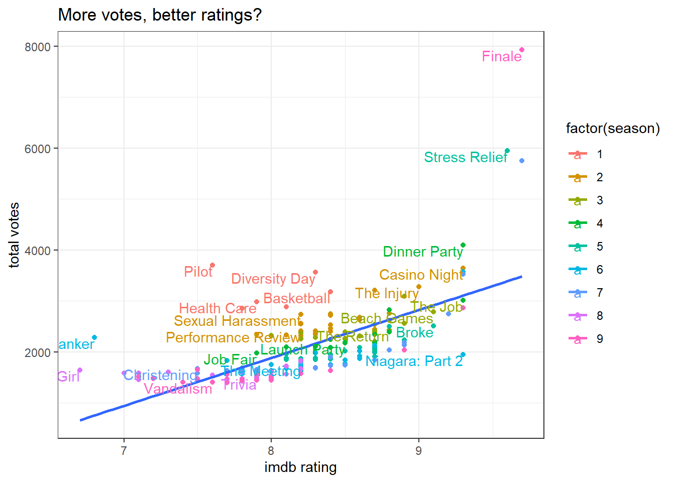
It seems like there is a positive relationship between IMDB rating and total # of votes. Maybe better episodes can attract more viewers to rate them!
office %>%
  ggplot(aes(air_date, imdb_rating, color = factor(season))) +
  geom_point() +
  geom_line() +
  geom_text(aes(label = total_votes), hjust = 1, vjust = 1, check_overlap = T) +
  scale_x_date(breaks = "1 year", date_labels = "%Y") +
  labs(x = "air year",
       y = "IMDB rating",
       color = "season",
       title = "How has the rating changed over time?")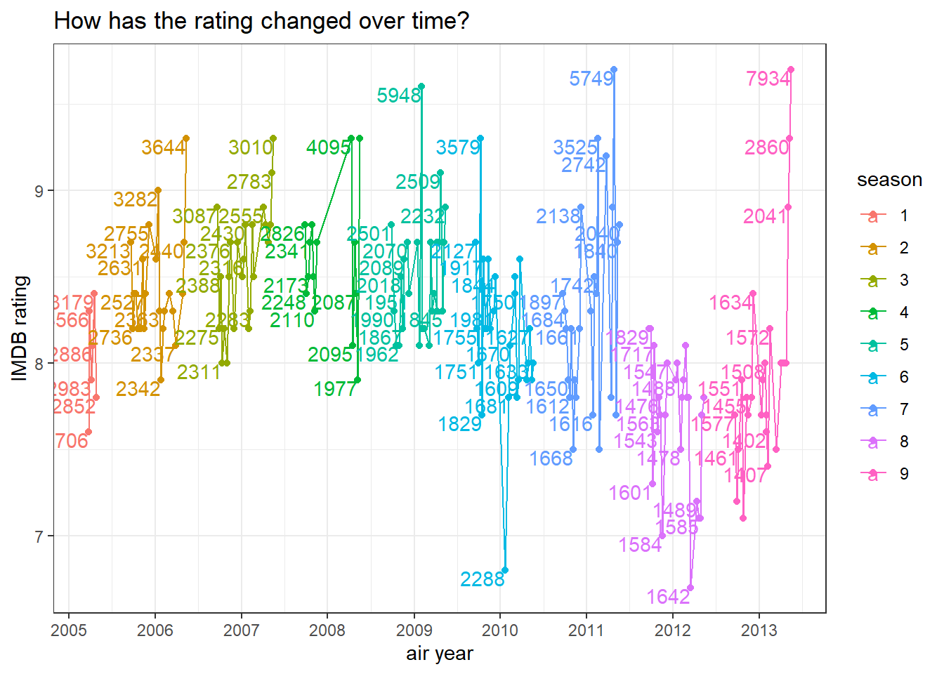
It seems like the year of 2010 had the wrost rating ever for one episode in Season 6.
office %>%
  mutate(season = paste("season", season)) %>%
  ggplot(aes(imdb_rating, season, fill = season)) +
  geom_boxplot(show.legend = F)  +
  labs(x = "IMDB rating",
       y = NULL,
       title = "Seasonal ratings")  +
  theme(axis.text = element_text(size = 13),
        plot.title = element_text(size = 18))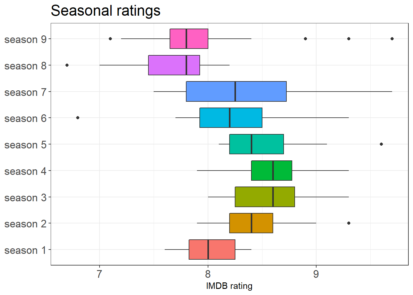
office %>%
  mutate(season = paste("season", season)) %>%
  ggplot(aes(total_votes, season, fill = season)) +
  geom_boxplot(show.legend = F)  +
  labs(x = "total votes",
       y = NULL,
       title = "Seasonal # of votes")  +
  theme(axis.text = element_text(size = 13),
        plot.title = element_text(size = 18))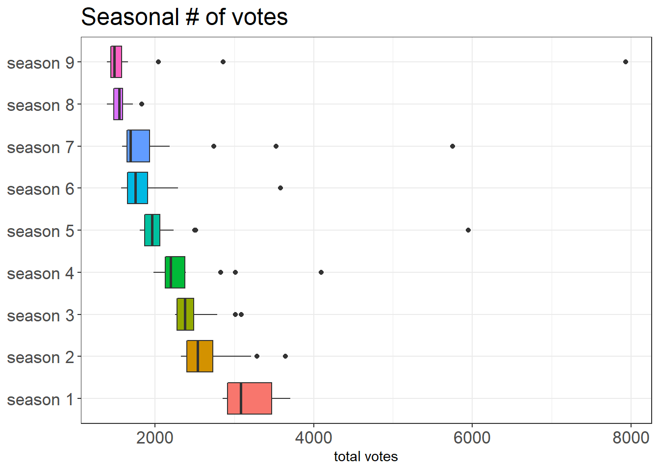
The vote boxplot gives us a different image in a way that there is a general decreasing voting trend when the show progressed.
title_matrix <- office %>%
  mutate(row_id = row_number()) %>%
  unnest_tokens(word, title) %>%
  anti_join(stop_words) %>%
  add_count(word) %>%
  cast_sparse(row_id, word)
## Joining, by = "word"Lasso model for predicting rating
# Lining up rating with row_id
row_id <- as.integer(rownames(title_matrix))

rating <- office$imdb_rating[row_id]

cv_glmnet_model <- cv.glmnet(title_matrix, rating)

plot(cv_glmnet_model)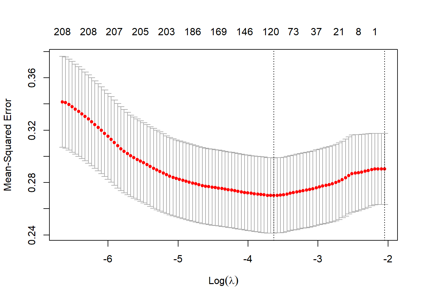
cv_glmnet_model$glmnet.fit %>%
  tidy() %>%
  filter(!str_detect(term, "(Intercept)"),
         lambda == cv_glmnet_model$lambda.min) %>%
  mutate(direction = if_else(estimate < 0, "negative", "positive")) %>%
  group_by(direction) %>%
  slice_max(abs(estimate), n = 20) %>%
  ungroup() %>%
  mutate(term = fct_reorder(term, estimate)) %>%
  ggplot(aes(estimate, term, fill = direction)) +
  geom_col(show.legend = F) +
  labs(title = "How does word in each episode impact its rating?")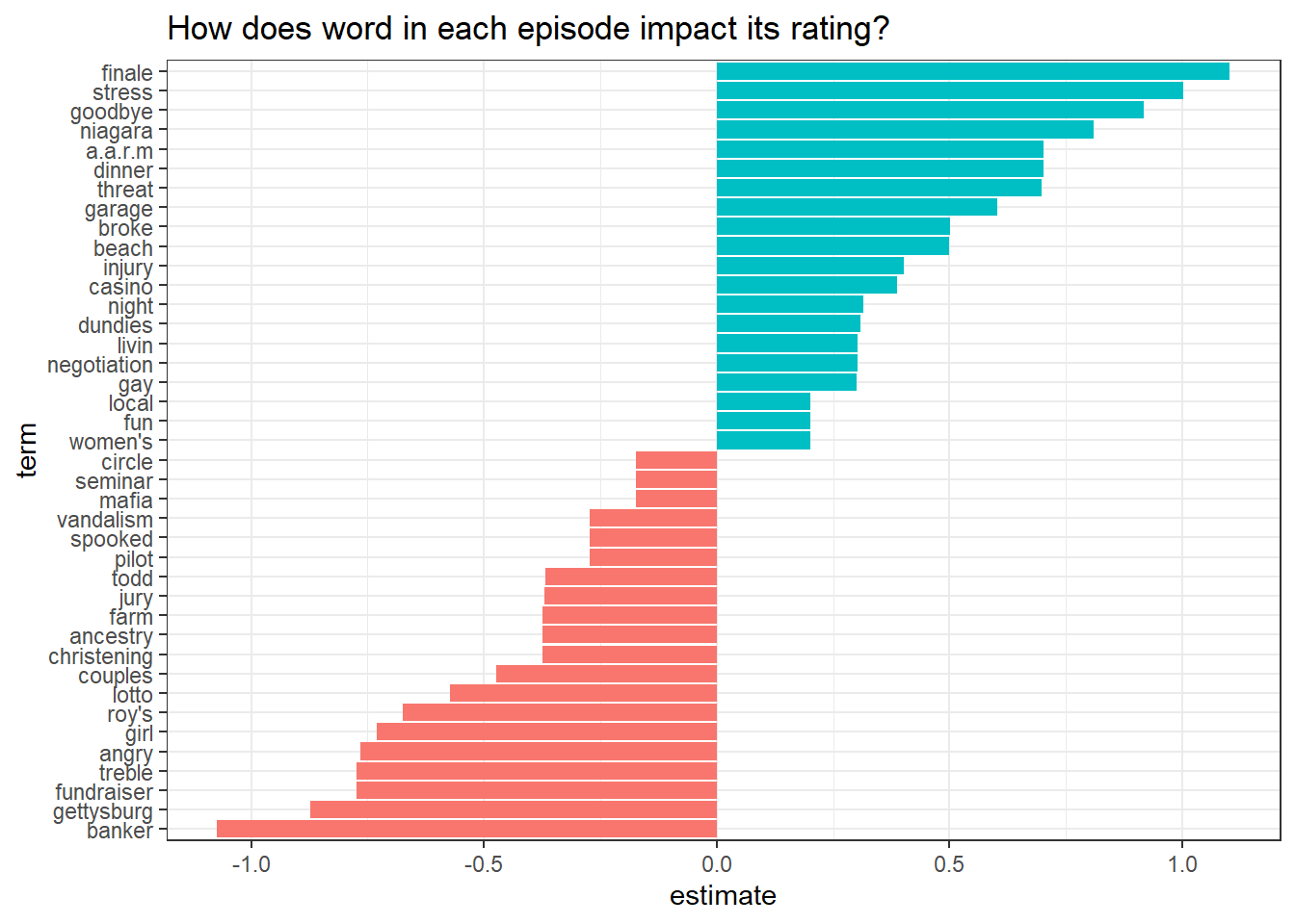
The Office transcripts from the schrute package
office_transcript <- schrute::theoffice %>%
  mutate(episode_name = str_remove(episode_name, " \\(Parts 1&2\\)"))
TF-IDF
TF stands for term frequency, and IDF inverse document frequency. Based on Chapter 3 of Text Mining with R (link), tf-idf provides a way to find the important words uniquely important to each character in this particular data analysis.
office_tf_idf <- office_transcript %>%
  mutate(row_id = row_number()) %>%
  unnest_tokens(word, text) %>%
  anti_join(stop_words) %>%
  count(character, word, sort = T) %>%
  bind_tf_idf(character, word, n) %>%
  arrange(desc(tf_idf)) %>%
  filter(n > 10)
## Joining, by = "word"top_10_characters <- office_transcript %>%
count(character, sort = T) %>%
head(9) %>%
pull(character)
office_tf_idf %>%
filter(character %in% top_10_characters) %>%
group_by(character) %>%
slice_max(tf_idf, n = 10, with_ties = F) %>%
ungroup() %>%
mutate(word = reorder_within(word, tf_idf, character)) %>%
ggplot(aes(tf_idf, word, fill = word)) +
geom_col(show.legend = F) +
scale_y_reordered() +
facet_wrap(~character, scales = "free_y") +
labs(x = "TF-IDF",
title = "Words from top 9 Characters that have the largest TF-IDF value")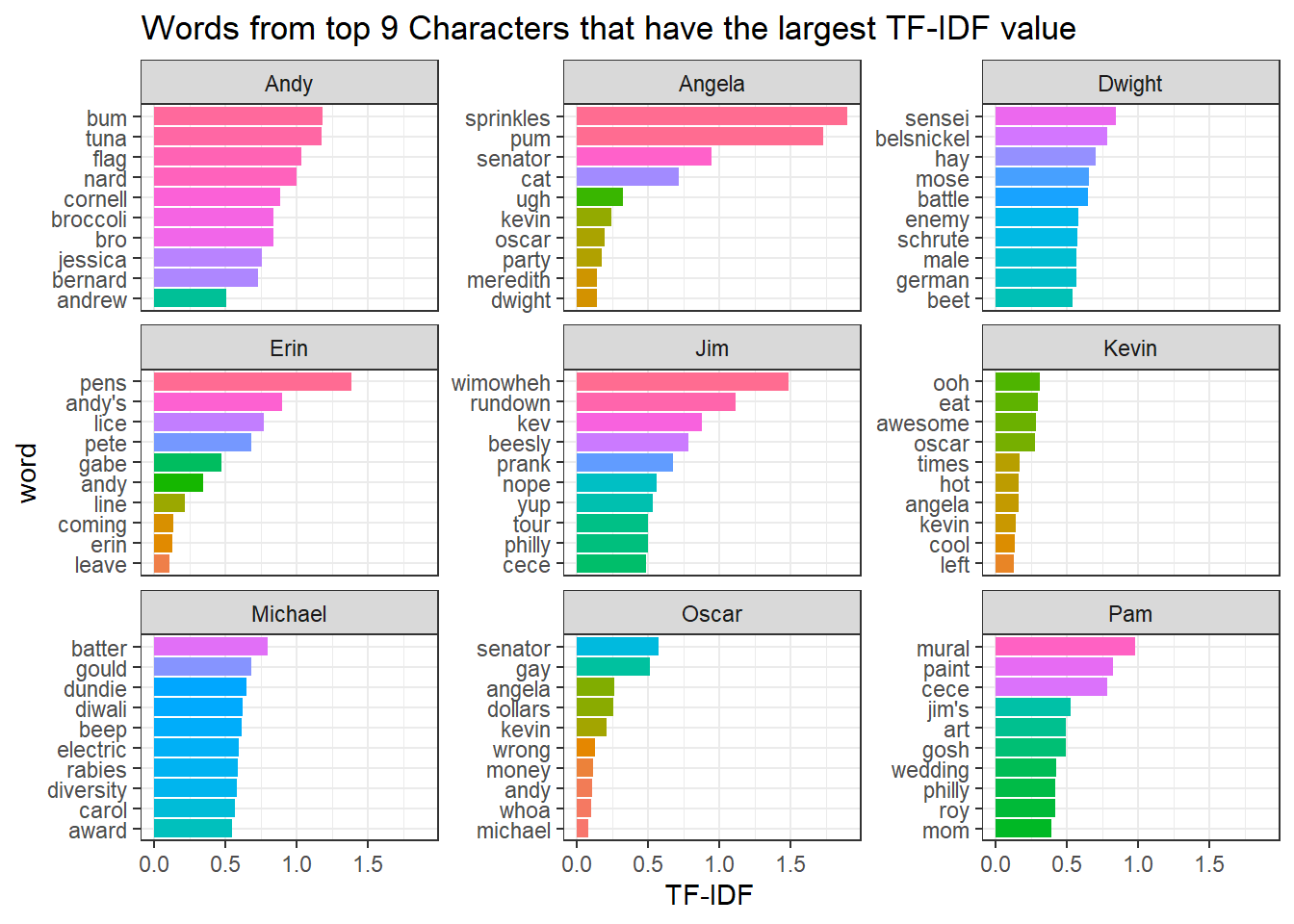
LASSO model
This model prediction is more advanced than the one shown above, as the model involves director, writer, and text line each character has, but the machine learning model is the same.
This section is inspired by David Robinson’s code. Here is the link.
I. Constructing features about directors and writers
director_writer_features <- office_transcript %>%
  distinct(episode_name, director, writer) %>%
  separate_rows(writer, sep = ";") %>%
  pivot_longer(cols = c(director, writer)) %>%
  mutate(feature = paste0(name,": ", value)) %>%
  select(episode_name, feature) %>%
  group_by(feature) %>%
  filter(n() > 5) %>%
  ungroup() %>%
  mutate(value = 1)


director_writer_features
## # A tibble: 309 x 3
## episode_name feature value
## <chr> <chr> <dbl>
## 1 Pilot director: Ken Kwapis 1
## 2 Pilot director: Ken Kwapis 1
## 3 Pilot director: Ken Kwapis 1
## 4 Pilot writer: Greg Daniels 1
## 5 Diversity Day director: Ken Kwapis 1
## 6 Diversity Day writer: B.J. Novak 1
## 7 Health Care director: Ken Whittingham 1
## 8 Health Care writer: Paul Lieberstein 1
## 9 The Alliance writer: Michael Schur 1
## 10 Basketball director: Greg Daniels 1
## # ... with 299 more rows- Constructing character line features
episode_summarized <- office_transcript %>%
               group_by(episode_name) %>%
               summarize(avg_rating = mean(imdb_rating)) %>%
  ungroup()


character_line_features <- office_transcript %>%
  count(episode_name, character, sort = T) %>%
  group_by(episode_name, character) %>%
  filter(sum(n) >= 50) %>%
  inner_join(episode_summarized) %>%
  ungroup() %>%
  transmute(episode_name, feature = character, value = log2(n))
## Joining, by = "episode_name"character_line_features## # A tibble: 244 x 3
## episode_name feature value
## <chr> <chr> <dbl>
## 1 Goodbye, Toby Michael 7.31
## 2 Launch Party Michael 7.20
## 3 Dunder Mifflin Infinity Michael 7.12
## 4 Money Michael 7.09
## 5 The Delivery Jim 7.07
## 6 Classy Christmas Michael 7.02
## 7 Fun Run Michael 7.02
## 8 Niagara Michael 7.01
## 9 The Delivery Pam 6.98
## 10 The Merger Michael 6.97
## # ... with 234 more rows- Constructing season features
season_features <- office_transcript %>%
  distinct(episode_name, season) %>%
  transmute(episode_name, feature = paste("season:", season), value = 1)

season_features
## # A tibble: 186 x 3
## episode_name feature value
## <chr> <chr> <dbl>
## 1 Pilot season: 1 1
## 2 Diversity Day season: 1 1
## 3 Health Care season: 1 1
## 4 The Alliance season: 1 1
## 5 Basketball season: 1 1
## 6 Hot Girl season: 1 1
## 7 The Dundies season: 2 1
## 8 Sexual Harassment season: 2 1
## 9 Office Olympics season: 2 1
## 10 The Fire season: 2 1
## # ... with 176 more rowsBinding all feature rows together
feature_matrix <- bind_rows(director_writer_features,
          character_line_features,
          season_features) %>%
  cast_sparse(episode_name, feature, value)

ratings <- episode_summarized$avg_rating[match(rownames(feature_matrix), episode_summarized$episode_name)]

lasso_model <- cv.glmnet(feature_matrix, ratings)

plot(lasso_model)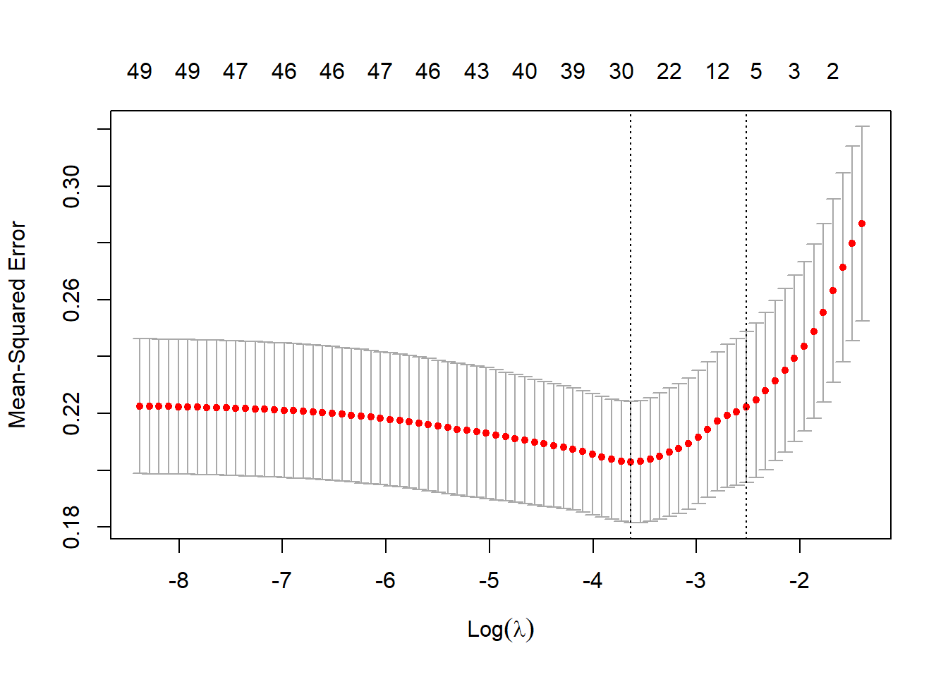
lasso_model$glmnet.fit %>%
  tidy() %>%
  filter(term != "(Intercept)",
         lambda == lasso_model$lambda.min) %>%
  mutate(term = fct_reorder(term, estimate)) %>%
  ggplot(aes(estimate, term, fill = estimate >0))+
  geom_col() +
  theme(legend.position = "none") +
  ggtitle("Lasso Model Prediction")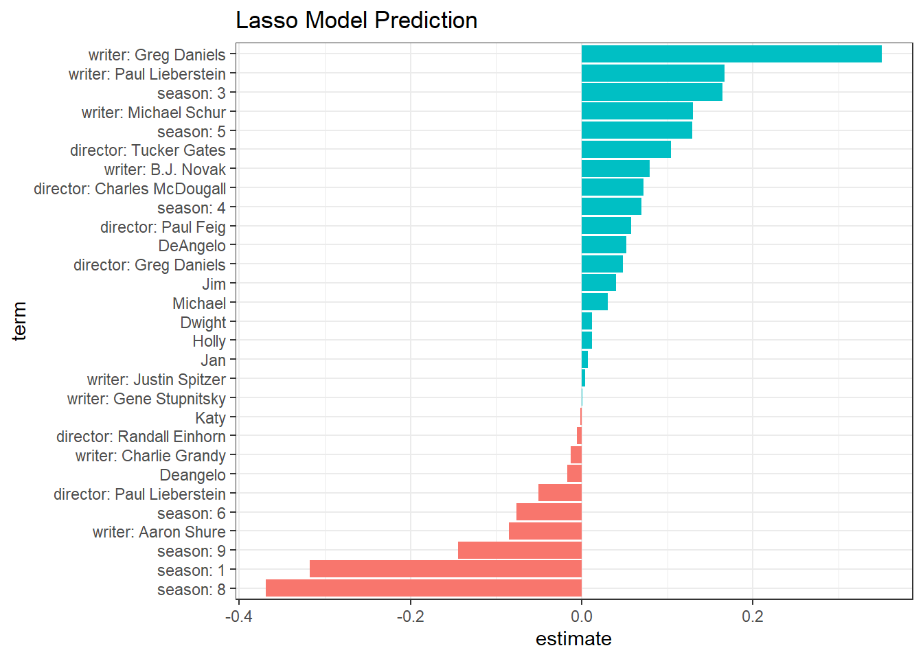
Greg Daniel as a writer contributes to the positive rating the most, and Season 8 might be contributing the wrost to the ratings.