Tour de France Data Visualization & Survival Analysis
This blog post analyzes datasets about Tour de France, which is the annual historical biking event held in France for more than 100 years. The datasets are from TidyTuesday.
library(tidyverse)
library(lubridate)
library(survival)
theme_set(theme_bw())
stage_data <- read_csv("https://raw.githubusercontent.com/rfordatascience/tidytuesday/master/data/2020/2020-04-07/stage_data.csv") %>%
mutate(decade = 10 * floor(year/10))
tdf_stages <- read_csv("https://raw.githubusercontent.com/rfordatascience/tidytuesday/master/data/2020/2020-04-07/tdf_stages.csv") %>%
janitor::clean_names() %>%
mutate(year = year(date))
tdf_winners <- read_csv("https://raw.githubusercontent.com/rfordatascience/tidytuesday/master/data/2020/2020-04-07/tdf_winners.csv") %>%
mutate(speed = distance / time_overall,
nationality = str_remove(nationality, "\\s"),
year = year(start_date))Working on stage_data
stage_data## # A tibble: 255,752 x 12
## edition year stage_results_id rank time rider age team points elapsed
## <dbl> <dbl> <chr> <chr> <chr> <chr> <dbl> <lgl> <dbl> <chr>
## 1 1 1903 stage-1 1 13S Garin ~ 32 NA 100 13S
## 2 1 1903 stage-1 2 55S Pagie ~ 32 NA 70 8S
## 3 1 1903 stage-1 3 59S George~ 23 NA 50 12S
## 4 1 1903 stage-1 4 48S Augere~ 20 NA 40 1S
## 5 1 1903 stage-1 5 53S Fische~ 36 NA 32 6S
## 6 1 1903 stage-1 6 53S Kerff ~ 37 NA 26 6S
## 7 1 1903 stage-1 7 55S Cattea~ 25 NA 22 8S
## 8 1 1903 stage-1 8 47S Pivin ~ 33 NA 18 0S
## 9 1 1903 stage-1 9 15S Habets~ NA NA 14 28S
## 10 1 1903 stage-1 10 26S Beauge~ 22 NA 10 39S
## # ... with 255,742 more rows, and 2 more variables: bib_number <lgl>,
## # decade <dbl>Yearly # of riders:
stage_data %>%
  distinct(year, rider, .keep_all = T) %>%
  count(year) %>%
  ggplot(aes(year, n)) +
  geom_line() +
  geom_smooth(method = "lm", se = F) +
  scale_x_continuous(breaks = seq(1900, 2020, 10)) +
  labs(y = "# of riders",
       title = "Yearly # of riders of Tour de France")
In terms of # of riders, there is an upward trend year by year.
stage_data %>%
  ggplot(aes(factor(decade), age, fill = factor(decade))) +
  geom_boxplot(show.legend = F) +
  labs(x = "decade",
       title = "The age of riders in each decade")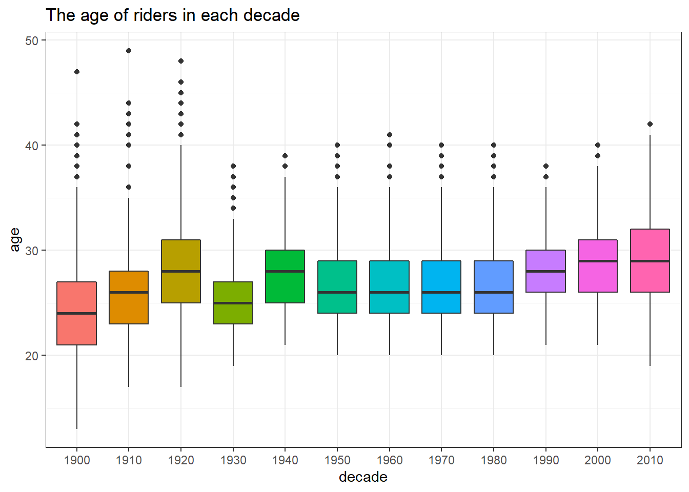
tdf_winners %>%
  mutate(year = year(start_date)) %>%
  ggplot(aes(year, speed)) +
  geom_line() +
  geom_point(aes(color = nationality)) +
  scale_x_continuous(breaks = seq(1900, 2020, 10)) +
  labs(y = "speed (km/h)",
       title = "Winner speed") +
  expand_limits(y = 0)
Clearly, the winner speed increased over the years. I assume this is in part due to the biking technological advancement, also in part because of the recent riders having the better training.
Winner citizenship status
tdf_winners %>%
  mutate(birth_nationality = if_else(birth_country == nationality, "Native", "Immigrant")) %>%
  ggplot(aes(birth_nationality)) +
  geom_histogram(stat = "count") +
  labs(x = NULL,
       title = "How many winners are native/immigrant?")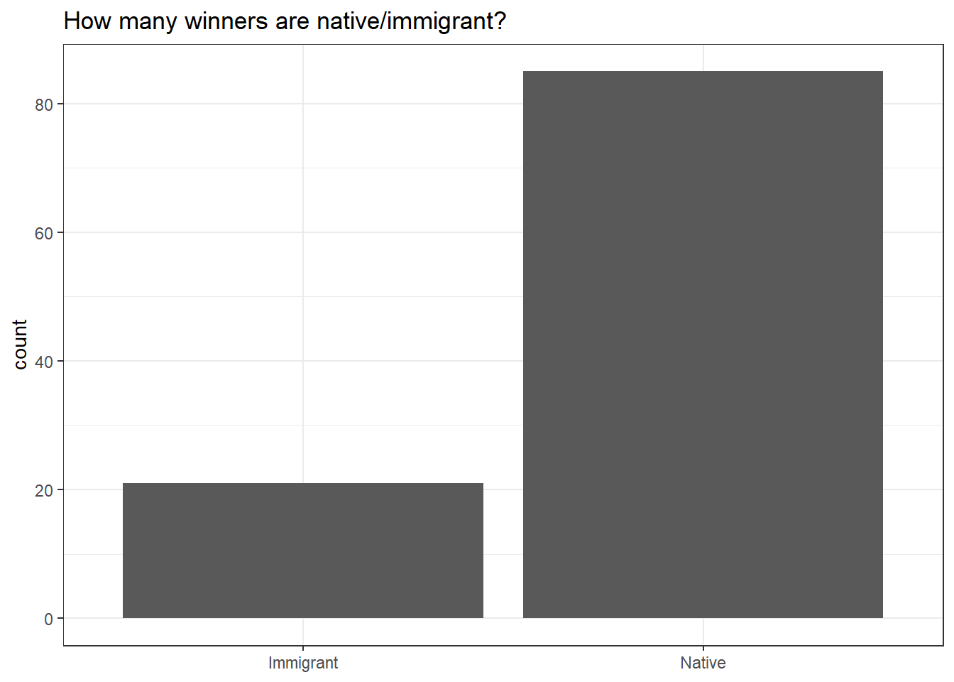
How long can winners live?
tdf_winners %>%
  mutate(life_age = round(difftime(died, born, units = "days")/365)) %>%
  ggplot(aes(start_date, life_age)) +
  geom_line() +
  expand_limits(y = 0) +
  labs(x = "year of winning",
       y = "life age",
       title = "How long can winners live?")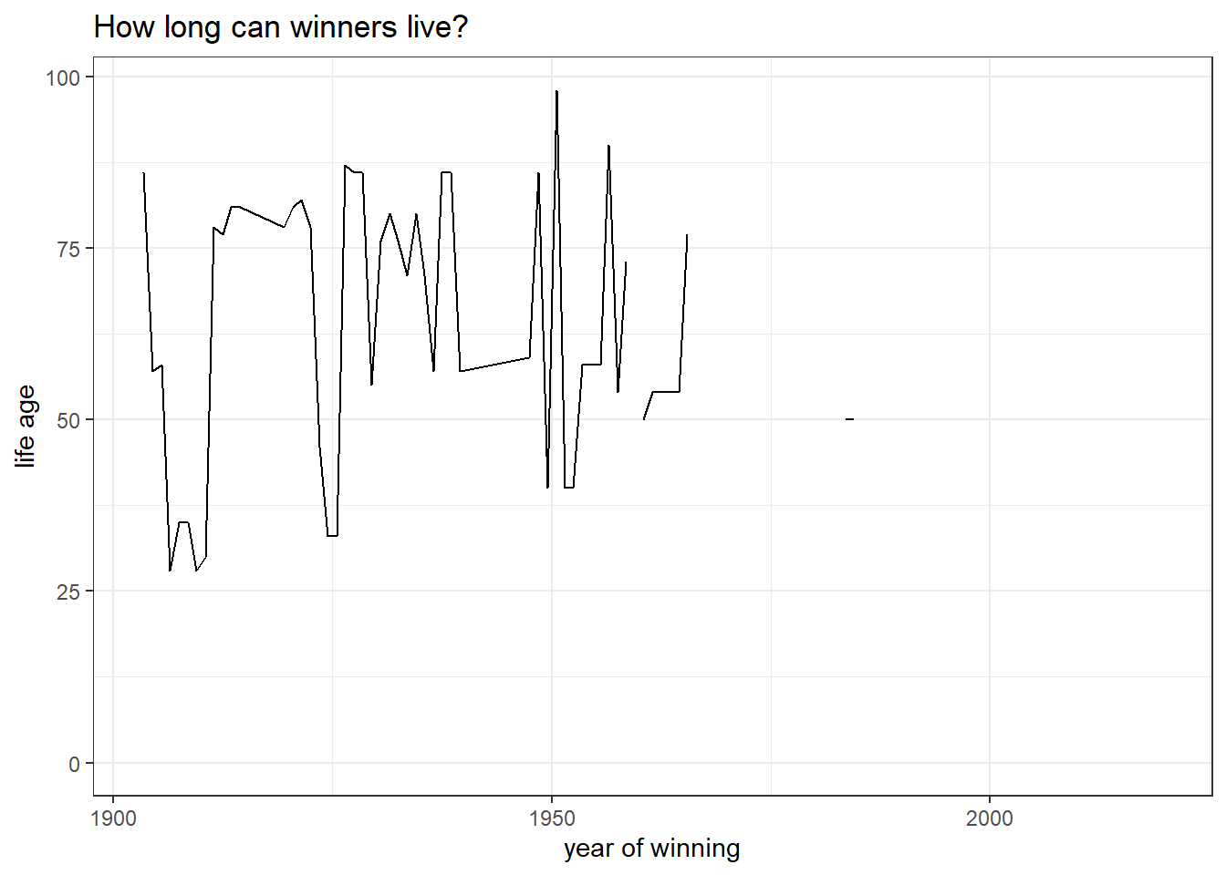
The above plot is misleading in a way that only dead winners are considered, as there are many winners who are still alive now.
Brief survival analysis
This little section is inspired by David Robinson’s code.
tdf_winners %>%
  distinct(winner_name, .keep_all = T) %>%
  transmute(winner_name,
            birth_year = year(born),
            death_year = year(died),
            dead = as.integer(!is.na(death_year))) %>%
  mutate(death_year = coalesce(death_year, 2021),
         age_at_death = death_year - birth_year) %>%
  survfit(Surv(age_at_death, dead) ~ 1, data = .)
## Call: survfit(formula = Surv(age_at_death, dead) ~ 1, data = .)
##
## n events median 0.95LCL 0.95UCL
## 63 38 77 71 82The median winner age is 77.
Join tdf_stages and tdf_winners together
tdf_joined <- tdf_stages %>%
  left_join(tdf_winners %>%
              select(year, final_winner = winner_name, total_distance = distance), by = "year")

tdf_joined
## # A tibble: 2,236 x 11
## stage date distance origin destination type winner winner_country
## <chr> <date> <dbl> <chr> <chr> <chr> <chr> <chr>
## 1 1 2017-07-01 14 Düsseldorf Düsseldorf Indi~ Gerai~ GBR
## 2 2 2017-07-02 204. Düsseldorf Liège Flat~ Marce~ GER
## 3 3 2017-07-03 212. Verviers Longwy Medi~ Peter~ SVK
## 4 4 2017-07-04 208. Mondorf-les-Bains Vittel Flat~ Arnau~ FRA
## 5 5 2017-07-05 160. Vittel La Planche~ Medi~ Fabio~ ITA
## 6 6 2017-07-06 216 Vesoul Troyes Flat~ Marce~ GER
## 7 7 2017-07-07 214. Troyes Nuits-Sain~ Flat~ Marce~ GER
## 8 8 2017-07-08 188. Dole Station de~ Medi~ Lilia~ FRA
## 9 9 2017-07-09 182. Nantua Chambéry High~ Rigob~ COL
## 10 10 2017-07-11 178 Périgueux Bergerac Flat~ Marce~ GER
## # ... with 2,226 more rows, and 3 more variables: year <dbl>,
## # final_winner <chr>, total_distance <dbl>tdf_joined %>%
mutate(stage_final_winner_match = if_else(winner == final_winner, TRUE, FALSE)) %>%
group_by(year) %>%
summarize(n = n(),
stage_wins_final_winner = sum(stage_final_winner_match),
winning_percent = stage_wins_final_winner/n) %>%
ggplot(aes(year, winning_percent)) +
geom_col() +
scale_y_continuous(labels = scales::percent) +
labs(y = "winning percentage",
title = "What is the percentage of the final winner winning stages by year?")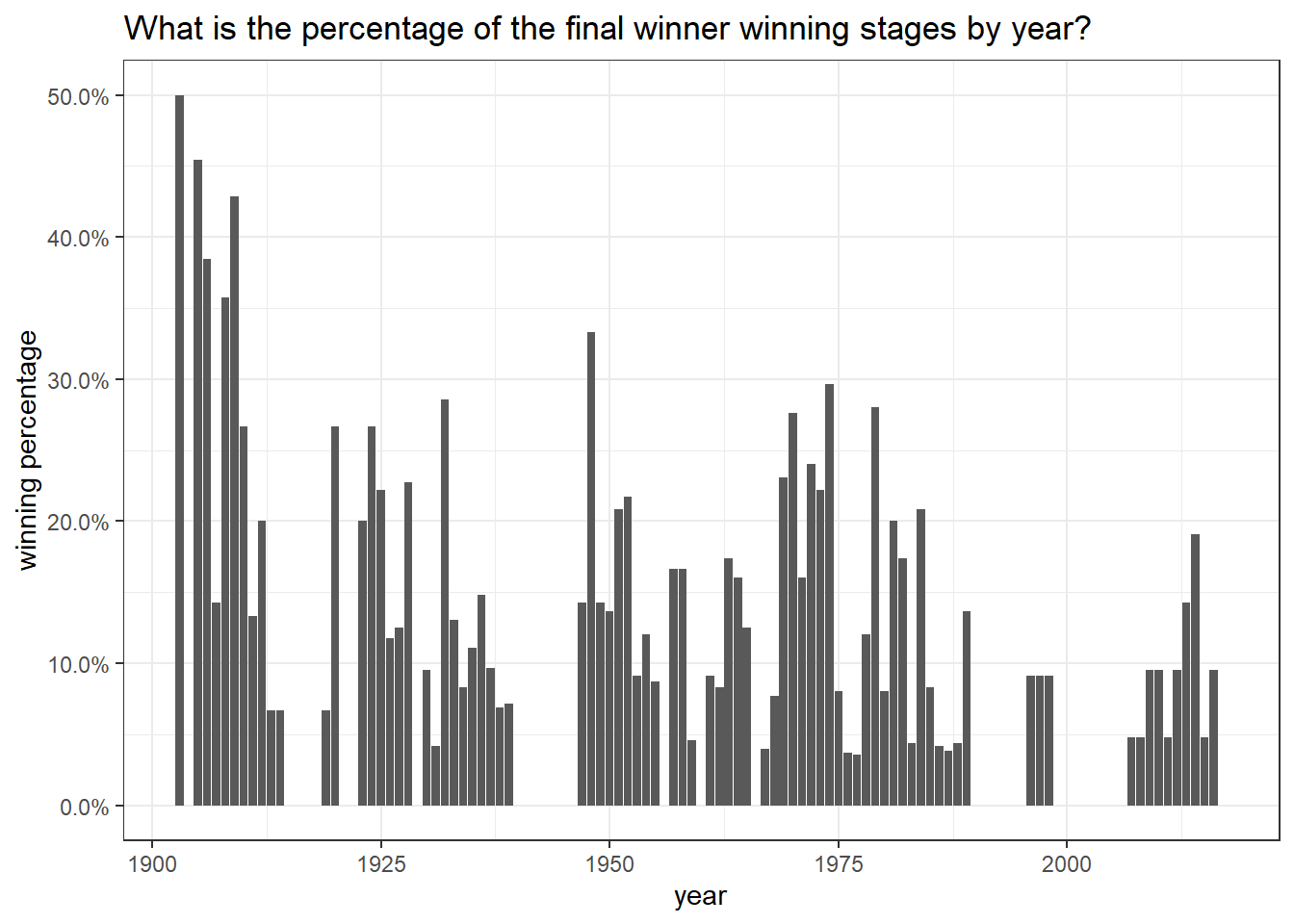
stage_joined <- stage_data %>%
  mutate(rank = as.numeric(rank)) %>%
  mutate(stage = str_remove(stage_results_id, "stage-")) %>%
  inner_join(tdf_stages %>%
              mutate(stage = as.character(stage)), by = c("stage", "year")) %>%
  group_by(year, stage) %>%
  mutate(finishers = n(),
         percentile = 1 - rank/finishers)
## Warning in mask$eval_all_mutate(quo): NAs introduced by coercionstage_joined## # A tibble: 242,022 x 22
## # Groups: year, stage [2,159]
## edition year stage_results_id rank time rider age team points elapsed
## <dbl> <dbl> <chr> <dbl> <chr> <chr> <dbl> <lgl> <dbl> <chr>
## 1 1 1903 stage-1 1 13S Garin ~ 32 NA 100 13S
## 2 1 1903 stage-1 2 55S Pagie ~ 32 NA 70 8S
## 3 1 1903 stage-1 3 59S George~ 23 NA 50 12S
## 4 1 1903 stage-1 4 48S Augere~ 20 NA 40 1S
## 5 1 1903 stage-1 5 53S Fische~ 36 NA 32 6S
## 6 1 1903 stage-1 6 53S Kerff ~ 37 NA 26 6S
## 7 1 1903 stage-1 7 55S Cattea~ 25 NA 22 8S
## 8 1 1903 stage-1 8 47S Pivin ~ 33 NA 18 0S
## 9 1 1903 stage-1 9 15S Habets~ NA NA 14 28S
## 10 1 1903 stage-1 10 26S Beauge~ 22 NA 10 39S
## # ... with 242,012 more rows, and 12 more variables: bib_number <lgl>,
## # decade <dbl>, stage <chr>, date <date>, distance <dbl>, origin <chr>,
## # destination <chr>, type <chr>, winner <chr>, winner_country <chr>,
## # finishers <int>, percentile <dbl>total_points <- stage_joined %>%
group_by(year, rider) %>%
summarize(total_points = sum(points, na.rm = TRUE)) %>%
mutate(points_rank = percent_rank(total_points)) %>%
ungroup()Does the first stage predict the total points?
stage_joined %>%
  inner_join(total_points, by = c("year", "rider")) %>%
  filter(stage == "1") %>%
  rename(first_stage_percentile = "percentile") %>%
  mutate(first_stage_bins = cut(first_stage_percentile, seq(0,1,0.1))) %>%
  filter(!is.na(first_stage_bins)) %>%
  ggplot(aes(points_rank, first_stage_bins)) +
  geom_boxplot() +
  labs(x = "total points percent rank",
       y = "first stage percentile",
       title = "Does the first stage predict the total points (performance)?") +
  scale_x_continuous(labels = scales::percent)
It looks like the first stage performance does impact how riders perform overall!