Broadway Weekly Grosses Data Visualization with tidymetrics

Adjusted price based on CPI

gross_cpi <- grosses %>%
  inner_join(cpi, by = c("year", "month")) %>%
  mutate(weekly_gross_overall_adj = 100 *weekly_gross_overall/cpi,
         weekly_gross_adj = 100 * weekly_gross/cpi,
         avg_ticket_price_adj = 100 * avg_ticket_price/cpi)

gross_cpi 

## # A tibble: 47,524 x 21
##    week_ending week_number weekly_gross_overall show     theatre    weekly_gross
##    <date>            <dbl>                <dbl> <chr>    <chr>             <dbl>
##  1 1985-06-09            1              3915937 42nd St~ St. James~       282368
##  2 1985-06-09            1              3915937 A Choru~ Sam S. Sh~       222584
##  3 1985-06-09            1              3915937 Aren't ~ Brooks At~       249272
##  4 1985-06-09            1              3915937 Arms an~ Circle in~        95688
##  5 1985-06-09            1              3915937 As Is    Lyceum Th~        61059
##  6 1985-06-09            1              3915937 Big Riv~ Eugene O'~       255386
##  7 1985-06-09            1              3915937 Biloxi ~ Neil Simo~       306839
##  8 1985-06-09            1              3915937 Brighto~ 46th Stre~       107392
##  9 1985-06-09            1              3915937 Cats     Winter Ga~       461880
## 10 1985-06-09            1              3915937 Doubles  Ritz Thea~        47452
## # ... with 47,514 more rows, and 15 more variables: potential_gross <dbl>,
## #   avg_ticket_price <dbl>, top_ticket_price <dbl>, seats_sold <dbl>,
## #   seats_in_theatre <dbl>, pct_capacity <dbl>, performances <dbl>,
## #   previews <dbl>, year <dbl>, month <dbl>, year_month <date>, cpi <dbl>,
## #   weekly_gross_overall_adj <dbl>, weekly_gross_adj <dbl>,
## #   avg_ticket_price_adj <dbl>

Gross revenue

gross_cpi  %>%
  distinct(week_ending, weekly_gross_overall_adj, .keep_all = T) %>%
  ggplot(aes(week_ending)) +
  geom_line(aes(y = weekly_gross_overall_adj, color = "adjusted gross")) +
  geom_line(aes(y = weekly_gross_overall, color = "non-adjusted gross")) +
  geom_smooth(aes(y = weekly_gross_overall_adj, color = "adjusted gross"), method = "lm", se = F) +
  geom_smooth(aes(y = weekly_gross_overall, color = "non-adjusted gross"), method = "lm", se = F) +
  labs(x = "year",
       y = "weekly box office overall gross",
       color = NULL,
       title = "Weekly box office gross (adjusted & unadjusted)") +
  scale_x_date(date_breaks = "5 years", date_labels = "%Y") +
  scale_y_continuous(label = dollar)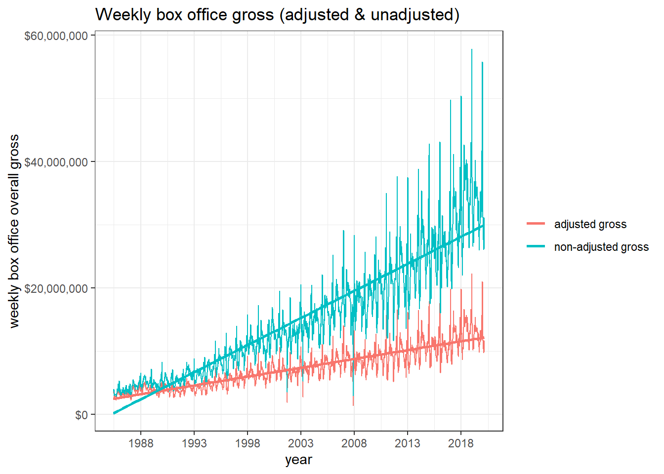

The gross revenue grew yearly, even when it is adjusted.

Average ticket price

top_5_shows <- gross_cpi %>%
  count(show, sort = T) %>%
  head(5) %>%
  pull(show)

gross_cpi %>%
  filter(show %in% top_5_shows) %>%
  ggplot(aes(avg_ticket_price_adj, theatre, fill = show)) +
  geom_boxplot() +
  scale_x_continuous(label = dollar) +
  labs(x = "ticket price (adjusted)",
       y = NULL,
       title = "Average ticket price for the top 5 popular shows")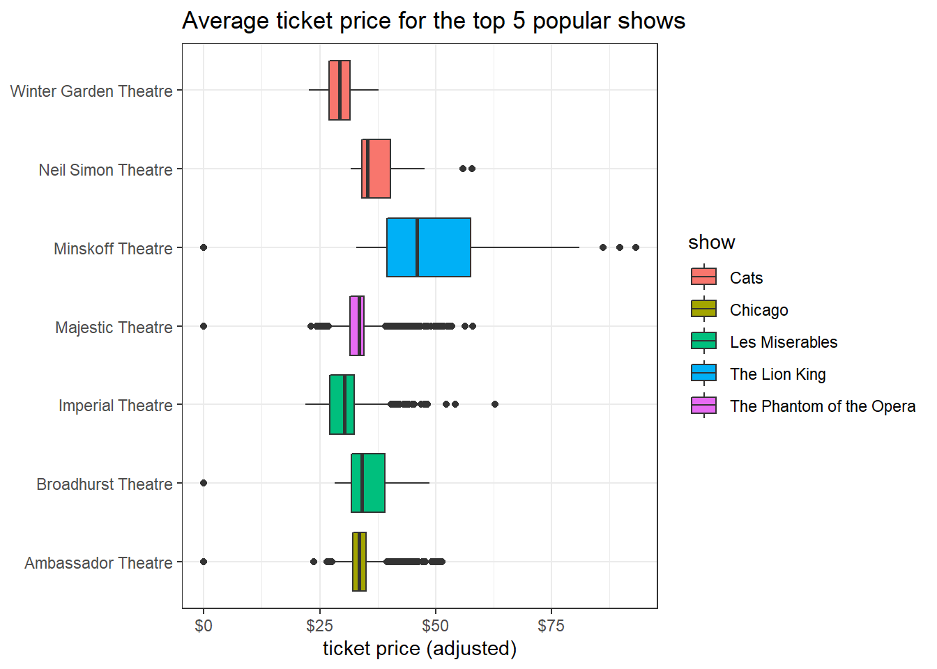

Average theatre capacity

gross_cpi %>%
  mutate(show = fct_lump(show, n = 30)) %>%
  filter(show != "Other") %>%
  group_by(show, theatre) %>%
  summarize(avg_cap = mean(pct_capacity),
            n = n()) %>%
  ungroup() %>%
  arrange(desc(n)) %>%
  head(100) %>%
  ggplot(aes(theatre, show)) +
  geom_point(aes(color = n, size = avg_cap)) +
  geom_text(aes(label = round(avg_cap, 1), color = n), size = 5, hjust = 1, vjust = 1, check_overlap = T) +
  theme(axis.text.x = element_text(angle = 90)) +
  labs(x = NULL,
       y = NULL,
       size = "average theatre capacity",
       color = "# of times the show in theatre",
       title = "30 Most Popular Shows Across Various Theatres") +
  scale_color_gradient2(low = "red",
                       high = "green",
                       mid = "pink",
                       midpoint = 800)

Tidymetrics

Here in this section, I am exploring the package tidymetrics, which is not on CRAN. You need to install it by devtools::install_github("datacamp/tidymetrics"). Also, this section is inspired by David Robinson's code. Otherwise, I would not even be aware of this package. gross_cpi is a wonderful dataset to harness this package.

gross_metrics <- gross_cpi %>%
  rename(date = "week_ending") %>%
  cross_by_periods(periods = c("month", "quarter", "year"),
                   windows = 28) %>%
  summarize(avg_price = mean(avg_ticket_price_adj),
            gross = sum(weekly_gross_overall_adj)) %>%
  ungroup()

gross_metrics %>%
  ggplot(aes(date, avg_price, color = period)) +
  geom_line(size = 1, alpha = 0.5) +
  labs(x = NULL,
       y = "average ticket price",
       title = "Average ticket price (adjusted) by month, quarter, and year") +
  scale_y_continuous(labels = dollar)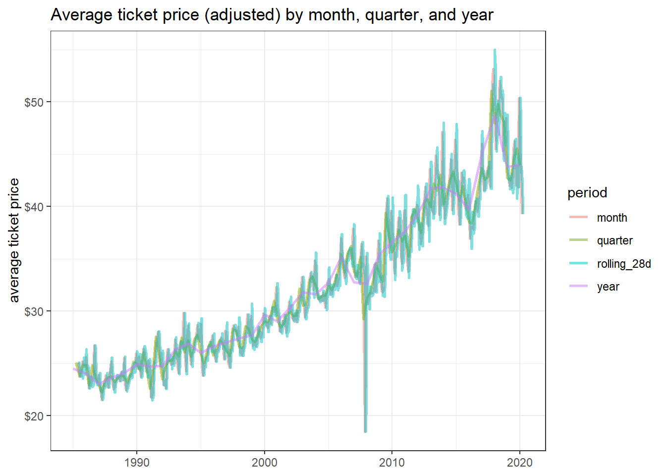

gross_metrics %>%
  ggplot(aes(date, gross, fill = period)) +
  geom_area(position = "stack") +
  facet_wrap(~period, ncol = 1) +
  theme(legend.position = "none",
        strip.text = element_text(size = 15),
        plot.title = element_text(size = 18)) +
  labs(x = NULL,
       y = "gross revenue",
       title = "Broadway adjusted grosss revenue") +
  scale_y_continuous(labels = dollar)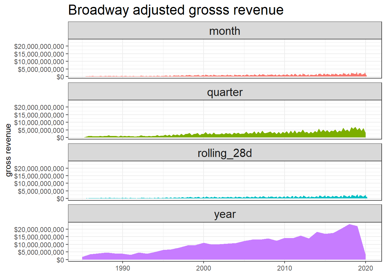

TF-IDF

by_words <- grosses %>%
  count(show, sort = T) %>%
  right_join(synopses, by = "show") %>%
  rename(show_times = "n") %>%
  unnest_tokens(word, synopsis) %>%
  anti_join(stop_words) %>%
  filter(!str_detect(word, "\\d+")) %>%
  add_count(show, word)


by_words %>%
  mutate(show = fct_lump(show, n = 12)) %>%
  filter(show != "Other",
         n > 1) %>%
  bind_tf_idf(word, show, n) %>%
  group_by(show) %>%
  slice_max(tf_idf, n = 1) %>%
  ungroup() %>%
  distinct(show, tf_idf, .keep_all = T) %>%
  mutate(word = fct_reorder(word, tf_idf)) %>%
  ggplot(aes(tf_idf, word, fill = show)) +
  geom_col() +
  labs(x = "TF-IDF",
       y = NULL,
       title = "The largest TF-IDF value for 12 most popular shows") +
  theme(axis.text = element_text(size = 12))