Beach Volleyball Data Visualization & Logistic Regression

Volleyable players' age

bv_longer %>%
  filter(str_detect(name, "age"),
         !is.na(round)) %>%
  mutate(round = fct_reorder(round, parse_number(round))) %>%
  ggplot(aes(as.numeric(value), winner_or_loser, fill = round)) +
  geom_boxplot() +
  facet_wrap(~round, ncol = 5) +
  theme(legend.position = "none") +
  labs(x = "age",
       y = "",
       title = "Age of winners and losers")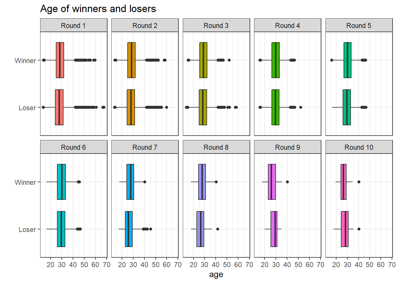

What is interesting is that there are people whose age is beyond 60 in Round 1. Other than that, the age difference between winner and loser is not obvious.

bv_longer %>%
  filter(str_detect(name, "hgt")) %>% 
  mutate(value = as.numeric(value)) %>%
  ggplot(aes(value, winner_or_loser, fill = winner_or_loser)) +
  geom_violin() +
  theme(legend.position = "none") +
  labs(x = "height (inches)",
       y = NULL,
       title = "The height of winners and losers")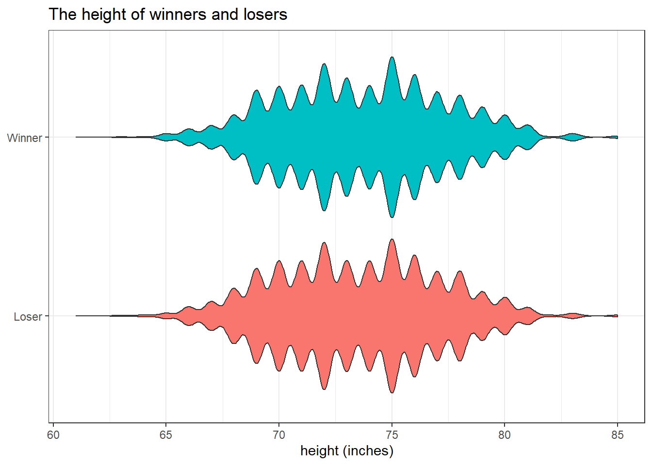

The distributions of height for winners and losers are almost identical.

Game duration

bv_longer %>%
  mutate(duration = hms(duration),
         round = fct_reorder(round, parse_number(round))) %>%
  distinct(match_num, duration, round) %>% 
  filter(!is.na(round)) %>%
  ggplot(aes(minute(duration), round)) +
  geom_boxplot() +
  labs(x = "duration (minutes)",
       y = NULL,
       title = "How long does game in each round take?")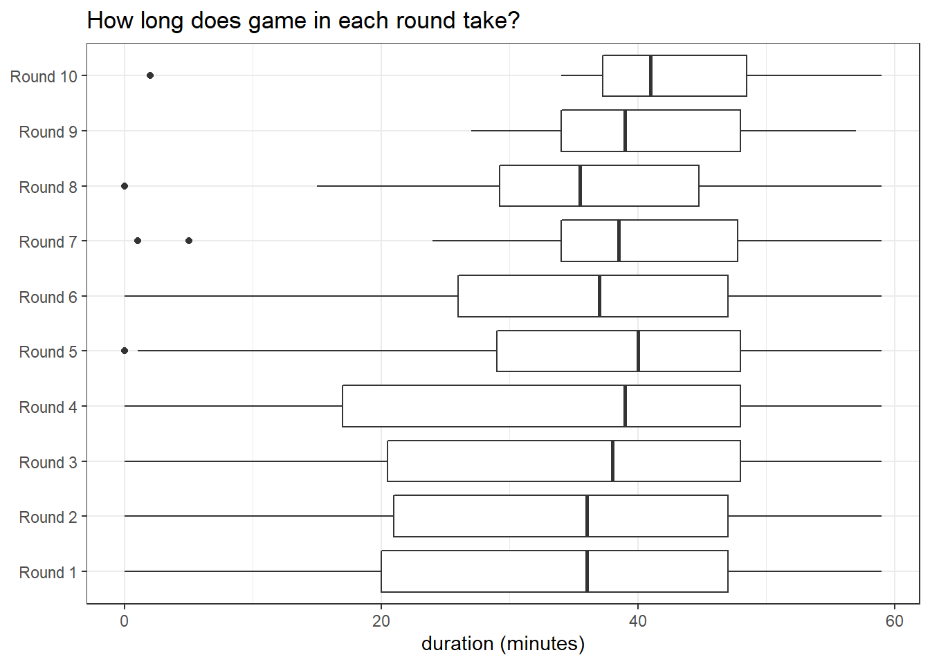

The final round

bv_longer %>%
  filter(str_detect(name, "country"),
         round == "Round 10") %>%
  count(value, winner_or_loser) %>%
  mutate(value = fct_reorder(value, n, sum)) %>%
  ggplot(aes(n, value, fill = winner_or_loser)) +
  geom_col() +
  scale_x_continuous(breaks = seq(0,13)) +
  labs(x = "# of wins or losses",
       y = NULL,
       fill = "",
       title = "Final Round (Round 10) Wins and Losses")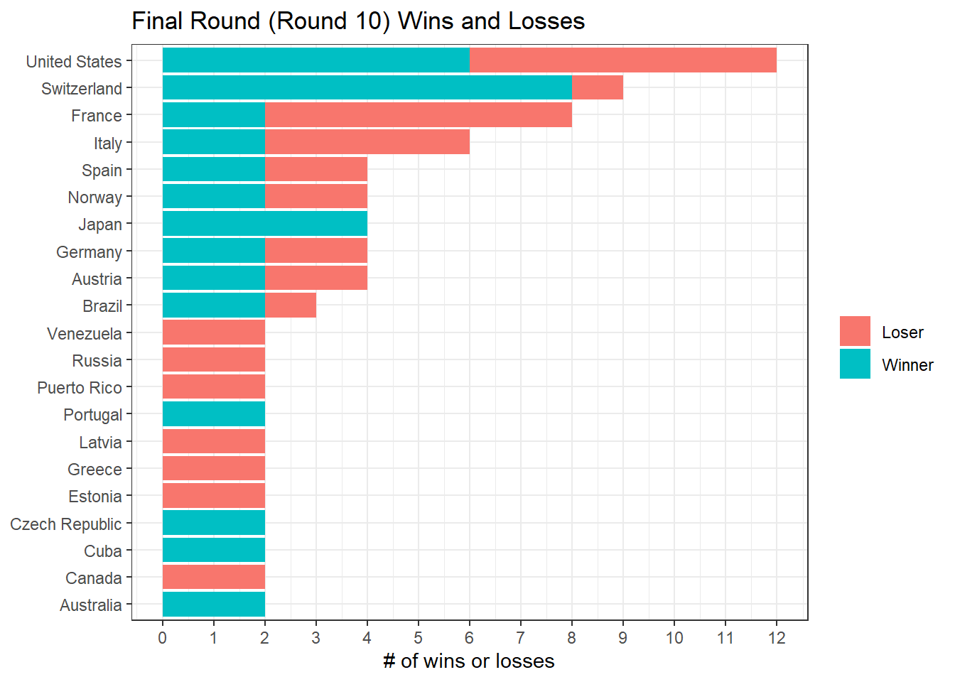

bv_longer_separate <- bv_longer %>%
  filter(!str_detect(name, "rank")) %>% 
  separate(name, into = c("win_or_lose","player", "variable"), sep = "_", extra = "merge", fill = "right") 

bv_spread <- bv_longer_separate %>%
  spread(key = "variable", value = "value") %>%
  type_convert()

bv_spread %>%
  summarize_all(~mean(is.na(.))) %>% 
  pivot_longer(everything()) 

## # A tibble: 26 x 2
##    name          value
##    <chr>         <dbl>
##  1 circuit    0       
##  2 tournament 0       
##  3 year       0       
##  4 date       0       
##  5 gender     0       
##  6 match_num  0       
##  7 score      0.000287
##  8 duration   0.0293  
##  9 bracket    0       
## 10 round      0.0643  
## # ... with 16 more rows

bv_spread <- bv_spread %>% 
  filter(!str_detect(score, "[:alpha:]"),
         !is.na(round)) %>%
  separate_rows(score, sep = ", ") %>%
  separate(score, into = c("win_score", "lose_score"), sep = "-", convert = TRUE) 

bv_spread %>% 
  distinct() %>%
  mutate(score_diff = win_score - lose_score,
         round = fct_reorder(round, parse_number(round))) %>% 
  ggplot(aes(abs(score_diff))) +
  geom_histogram() +
  facet_wrap(~round, scales = "free_y", ncol = 2) +
  scale_x_continuous(breaks = seq(1,20)) +
  labs(x = "score difference",
       title = "Score difference across all rounds") 

The scores are rather close, as we can see there are many games in each round whose difference is 2 or 3.

I would like to acknowledge that the following chunk of code is inspired by David Robinson's code.

by_player <- bv_spread %>% 
  group_by(name, gender) %>%
  summarize(n_matches = n(),
            pct_winner = mean(win_or_lose == "w"),
            first_game = min(date),
            last_game = max(date)) %>%
  arrange(desc(n_matches)) %>%
  ungroup() 

by_player %>%
  filter(n_matches > 100) %>%
  ggplot(aes(pct_winner, n_matches, color = gender)) +
  geom_point() +
  scale_x_log10(label = scales::percent) +
  scale_y_log10() +
  labs(x = "winning percentage",
       y = "# of matches",
       title = "The relation between winning and # of matches",
       subtitle = "Only players who played more than 100 games are considered")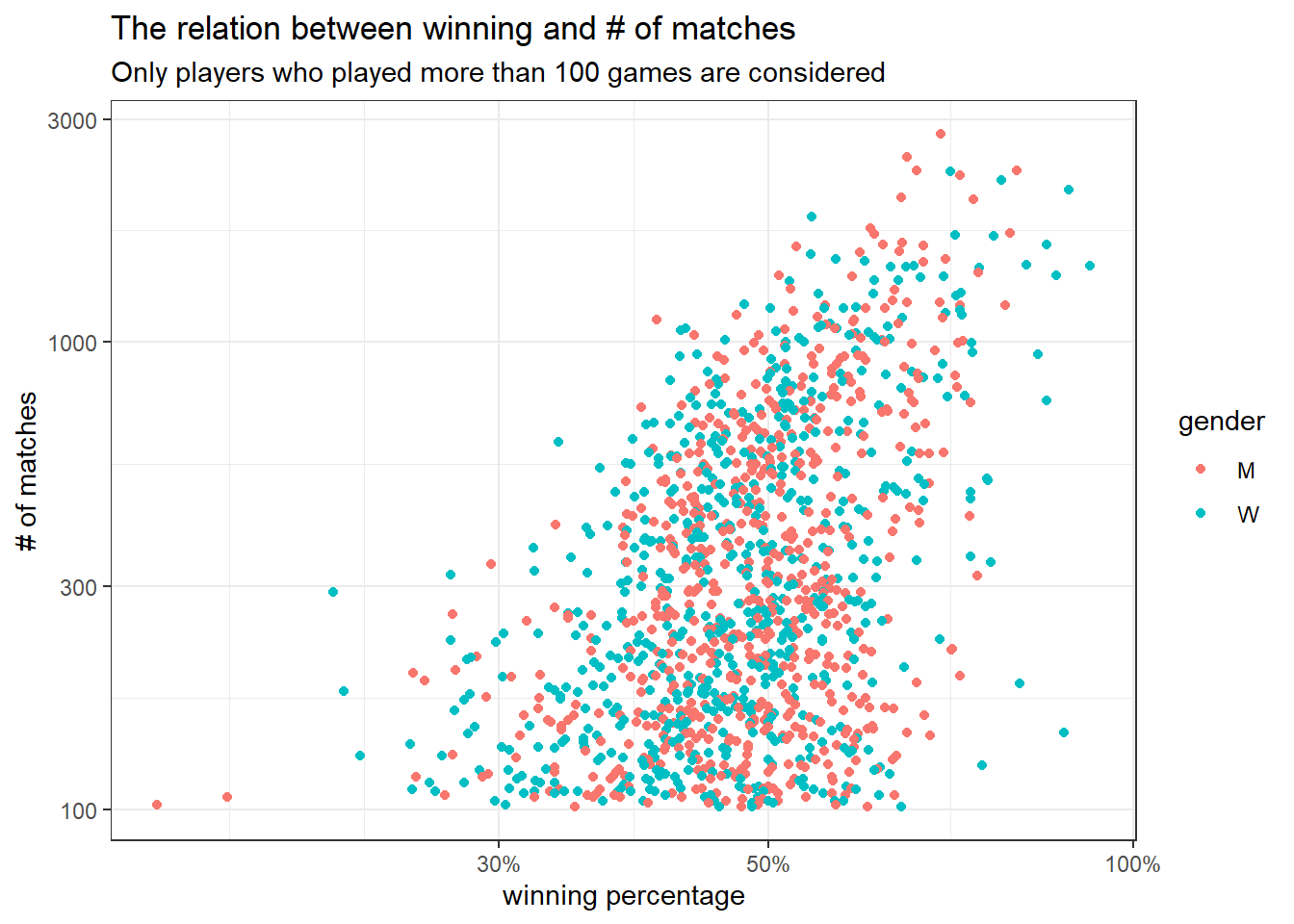

Data processing

summarize_players <- . %>%
  summarize(n_matches = n(),
            pct_winner = mean(win_or_lose == "w"),
            avg_attacks = mean(tot_attacks, na.rm = TRUE),
            avg_errors = mean(tot_errors, na.rm = TRUE),
            avg_serve_errors = mean(tot_serve_errors, na.rm = TRUE),
            avg_kills = mean(tot_kills, na.rm = TRUE),
            avg_aces = mean(tot_aces, na.rm = TRUE),
            n_with_data = sum(!is.na(tot_attacks))) %>%
  ungroup() %>%
  arrange(desc(n_matches))

players_before_2019 <- bv_spread %>%
  filter(year < 2019) %>%
  group_by(name, gender, hgt, birthdate, country) %>%
  summarize_players() %>%
  filter(!is.na(avg_attacks))

players_2019 <- bv_spread %>%
  filter(year == 2019) %>%
  group_by(name, gender, hgt, birthdate, country, year,
           age = year - year(birthdate)) %>%
  summarize_players()

joined <- players_before_2019 %>%
  inner_join(players_2019 %>%
               select(name, pct_winner, n_matches),
             by = "name",
             suffix = c("", "_2019"))

joined %>% 
  ggplot(aes(pct_winner, pct_winner_2019, color = gender)) +
  geom_point() +
  geom_smooth(method = "lm", se = F, aes(group = 1)) +
  geom_text(aes(label = name), hjust = 1, vjust = 1, check_overlap = T) +
  labs(x = "wining percentage before 2019",
       y = "winning percentage in 2019",
       title = "Winning percentage before and in 2019") +
  scale_x_continuous(label = scales::percent) +
  scale_y_continuous(label = scales::percent)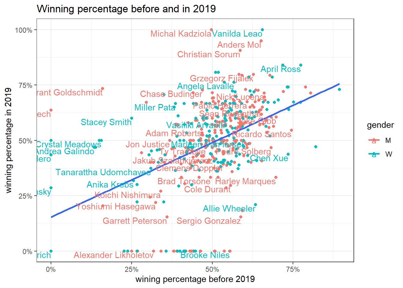 

We can fit a logistic regression with cbind().

joined %>%
  mutate(n_wins_2019 = n_matches_2019 * pct_winner_2019) %>%
  glm(cbind(n_wins_2019, n_matches_2019 - n_wins_2019) ~ pct_winner + avg_errors + avg_serve_errors,
      data = .,
      family = "binomial") %>% 
  tidy() %>%
  filter(term != "(Intercept)") %>%
  ggplot(aes(y = term)) +
  geom_point(aes(x = estimate)) +
  geom_errorbarh(aes(xmin = estimate - std.error,
                 xmax = estimate + std.error))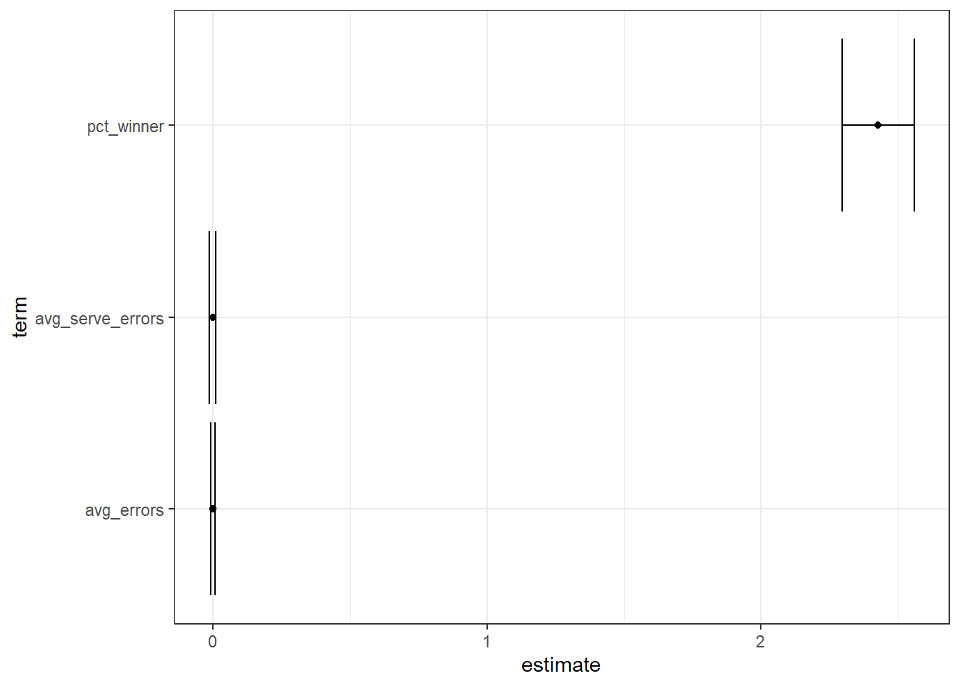 

Only pct_winner the pervious winning percentage before 2019 has a significant impact to the player winning percentage in 2019.