African-American Achievements Data Processing & Visualization
Wed, Jan 12, 2022
5-minute read
This blog post analyzes the African-American achievements data sets from TidyTuesday. The data sets are webscraped from Wikipeida and some preprocessing steps are needed in order to visualize the data.
library(tidyverse)
library(tidytext)
library(widyr)
library(ggraph)
library(igraph)
theme_set(theme_bw())
firsts <- read_csv('https://raw.githubusercontent.com/rfordatascience/tidytuesday/master/data/2020/2020-06-09/firsts.csv') %>%
mutate(first_accomplishment = str_trim(str_remove_all(accomplishment, "First|African.?American"), "left"),
decade = 10 * floor(year/10))
science <- read_csv('https://raw.githubusercontent.com/rfordatascience/tidytuesday/master/data/2020/2020-06-09/science.csv')
firsts## # A tibble: 479 x 7
## year accomplishment person gender category first_accomplish~ decade
## <dbl> <chr> <chr> <chr> <chr> <chr> <dbl>
## 1 1738 First free Africa~ Gracia Re~ Africa~ Social ~ free community 1730
## 2 1760 First known Afric~ Jupiter H~ Female~ Arts & ~ known published~ 1760
## 3 1768 First known Afric~ Wentworth~ Africa~ Social ~ known to be ele~ 1760
## 4 1773 First known Afric~ Phillis W~ Female~ Arts & ~ known woman to ~ 1770
## 5 1773 First separate Af~ Silver Bl~ Africa~ Religion separate church 1770
## 6 1775 First African-Ame~ Prince Ha~ Africa~ Social ~ to join the Free~ 1770
## 7 1778 First African-Ame~ the 1st R~ Africa~ Military U.S. military re~ 1770
## 8 1783 First African-Ame~ James Der~ Africa~ Educati~ to formally prac~ 1780
## 9 1785 First African-Ame~ Rev. Lemu~ Africa~ Religion ordained as a Ch~ 1780
## 10 1792 First major Afric~ 3,000 Bla~ Africa~ Social ~ major Back-to-A~ 1790
## # ... with 469 more rowsscience## # A tibble: 120 x 7
## name birth death occupation_s inventions_accompli~ references links
## <chr> <dbl> <dbl> <chr> <chr> <chr> <chr>
## 1 Amos, ~ 1918 2003 Microbiologist First African-Ameri~ 6, https://~
## 2 Alcorn~ 1940 NA Physicist; inv~ Invented a method o~ 7,8, https://~
## 3 Andrew~ 1930 1998 Mathematician Put forth the Andre~ 9, https://~
## 4 Alexan~ 1888 1958 Civil engineer Responsible for the~ <NA> https://~
## 5 Bailey~ 1825 1918 Inventor Folding bed 10, https://~
## 6 Ball, ~ 1892 1916 Chemist Extracted chaulmoog~ 11, https://~
## 7 Bannek~ 1731 1806 Almanac author~ Constructed wooden ~ 12, https://~
## 8 Banyag~ 1947 NA Mathematician Work on diffeomorph~ 13, https://~
## 9 Bashen~ 1957 NA Inventor; entr~ First African-Ameri~ 14, https://~
## 10 Bath, ~ 1942 2019 Ophthalmologist First African-Ameri~ 15,16,17, https://~
## # ... with 110 more rowsWorking on the firsts tibble
firsts %>%
  group_by(decade, category) %>%
  summarize(n = n()) %>%
  ungroup() %>%
  ggplot(aes(decade, n, fill = category)) +
  geom_col() +
  scale_x_continuous(breaks = seq(1700, 2000, 50)) +
  scale_y_continuous(breaks = seq(0,60,10)) +
  labs(y = "# of first achievement",
       title = "Category-wise first African American achievements from 1730s to 2010s")
African-American accomplishment description TF-IDF among all categories
firsts %>%
  unnest_tokens(word, first_accomplishment) %>%
  anti_join(stop_words) %>%
  filter(!str_detect(word, "[:digit:]")) %>%
  count(word, category) %>%
  bind_tf_idf(word, category, n) %>%
  group_by(category) %>%
  slice_max(tf_idf, n = 10) %>%
  ungroup() %>%
  mutate(word = reorder_within(word, tf_idf, category)) %>%
  ggplot(aes(tf_idf, word, fill = category)) +
  geom_col() +
  scale_y_reordered() +
  facet_wrap(~category, scales = "free_y", ncol = 4) +
  theme(legend.position = "none",
        strip.text = element_text(size = 12),
        axis.text.y = element_text(size = 12)) +
  labs(x = "TF-IDF",
       y = NULL,
       title = "The 10 largest categorical TF-IDF values")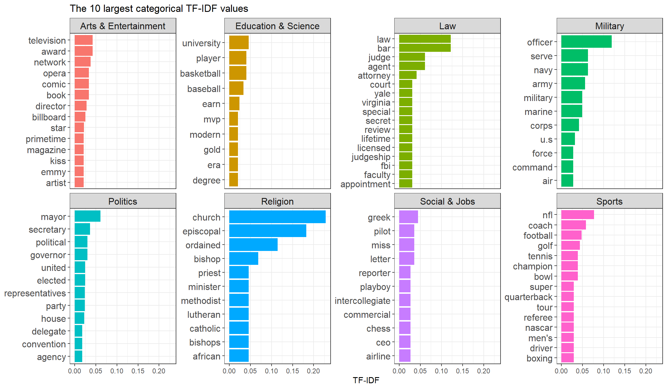
Now let's work on science.
science_processed <- science %>%
  separate(name, into = c("last_name", "first_name"), sep = ", ") %>%
  separate_rows(occupation_s, sep = ";\\s+") %>%
  rename(occuption = "occupation_s") %>%
  mutate(occuption = str_to_title(occuption),
         full_name = paste(first_name, last_name),
         alive_or_dead = if_else(is.na(death), "Alive", "Dead"),
         age = if_else(is.na(death), 2022 - birth, death - birth)) %>%
  select(-c(references, links))

science_processed
## # A tibble: 164 x 9
## last_name first_name birth death occuption inventions_acco~ full_name
## <chr> <chr> <dbl> <dbl> <chr> <chr> <chr>
## 1 Amos Harold 1918 2003 Microbiologist First African-A~ Harold A~
## 2 Alcorn George Edward 1940 NA Physicist Invented a meth~ George E~
## 3 Alcorn George Edward 1940 NA Inventor Invented a meth~ George E~
## 4 Andrews James J. 1930 1998 Mathematician Put forth the A~ James J.~
## 5 Alexander Archie 1888 1958 Civil Engineer Responsible for~ Archie A~
## 6 Bailey Leonard C. 1825 1918 Inventor Folding bed Leonard ~
## 7 Ball Alice Augusta 1892 1916 Chemist Extracted chaul~ Alice Au~
## 8 Banneker Benjamin 1731 1806 Almanac Author Constructed woo~ Benjamin~
## 9 Banneker Benjamin 1731 1806 Surveyor Constructed woo~ Benjamin~
## 10 Banneker Benjamin 1731 1806 Farmer Constructed woo~ Benjamin~
## # ... with 154 more rows, and 2 more variables: alive_or_dead <chr>, age <dbl>science_processed %>%
mutate(occuption = fct_lump(occuption, n = 10)) %>%
filter(!is.na(occuption),
age < 100) %>%
ggplot(aes(age, occuption, fill = alive_or_dead)) +
geom_boxplot() +
scale_x_continuous(breaks = seq(20, 100, 20)) +
labs(y = NULL,
fill = NULL,
title = "Age among all people presented in science_processed",
subtitle = "The age of people who fall into the Alive category is computed by using 2022 - their birth year") +
theme(axis.text = element_text(size = 10),
axis.title = element_text(size = 13),
plot.title = element_text(size = 15))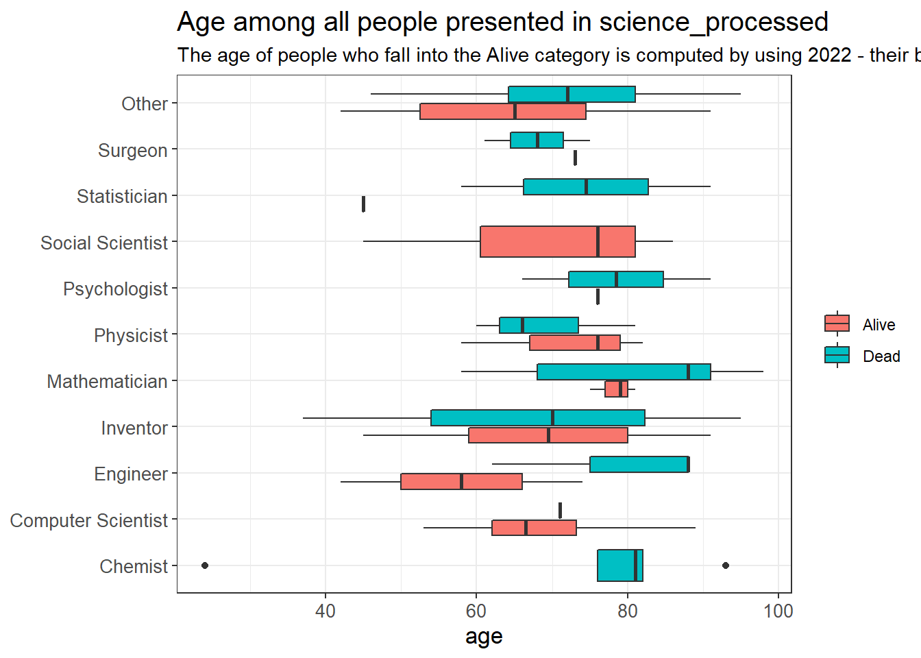
set.seed(2022)

science_processed %>%
  add_count(occuption) %>%
  filter(n > 2) %>%
  pairwise_cor(occuption, full_name, sort = T) %>%
  graph_from_data_frame() %>%
  ggraph(layout = "fr") +
  geom_edge_link(aes(color = correlation > 0, width  = abs(correlation))) +
  geom_node_point() +
  geom_node_text(aes(label = name), vjust = 1, hjust = 1, size = 5) +
  theme_void() +
  guides(edge_width = "none") +
  ggtitle("How are different occuptions linked together?") +
  theme(plot.title = element_text(size = 15))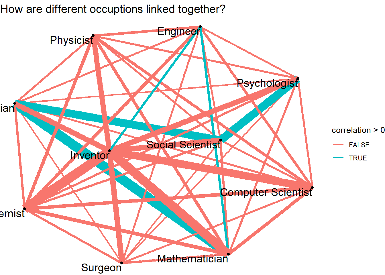
It is very interesting to see how the occuption(s) each person has are linked together. Statistican and mathematician are strongly positively correlated, but it seems like mathematician is slightly and negatively correlated with social scientist. You can come up with many interesting findings from the graph above!