X-men Data Visualization (Lollipop Plot included)
The data sets about X-men for this blog post come from TidyTuesday. Instead of loding them manually this time, I will use the tidytuesdayR package. You can install it by simply typing install.packages("tidytuesdayR") on your console!
Before doing any data analysis, I do need to admit that I don't know anything about X-men, meaning there is no any background information I hold. This blog post is just simply about analyzing data.
Now load the packages!
library(tidyverse)
library(tidytuesdayR)
library(ggraph)
library(tidytext)
library(cowplot)
theme_set(theme_bw())
tt_load() is the way to load the data sets.
#tuesdata <- tidytuesdayR::tt_load('2020-06-30')Or you can read them manually.
comic_bechdel <- read_csv('https://raw.githubusercontent.com/rfordatascience/tidytuesday/master/data/2020/2020-06-30/comic_bechdel.csv')

character_visualization <- read_csv('https://raw.githubusercontent.com/rfordatascience/tidytuesday/master/data/2020/2020-06-30/character_visualization.csv')

characters <- read_csv('https://raw.githubusercontent.com/rfordatascience/tidytuesday/master/data/2020/2020-06-30/characters.csv')

xmen_bechdel <- read_csv('https://raw.githubusercontent.com/rfordatascience/tidytuesday/master/data/2020/2020-06-30/xmen_bechdel.csv')

locations <- readr::read_csv('https://raw.githubusercontent.com/rfordatascience/tidytuesday/master/data/2020/2020-06-30/locations.csv')
Analyzing character_visualization
character_visualization  <- character_visualization %>%
  mutate(character = str_remove_all(character, "\\s.+|/.+|\\s?=.+"))
character_visualization
## # A tibble: 9,800 x 7
## issue costume character speech thought narrative depicted
## <dbl> <chr> <chr> <dbl> <dbl> <dbl> <dbl>
## 1 97 Costume Editor 0 0 0 0
## 2 97 Costume Omnipresent 0 0 0 0
## 3 97 Costume Professor 0 0 0 0
## 4 97 Costume Wolverine 7 0 0 10
## 5 97 Costume Cyclops 24 3 0 23
## 6 97 Costume Marvel 0 0 0 0
## 7 97 Costume Storm 11 0 0 9
## 8 97 Costume Colossus 9 0 0 17
## 9 97 Costume Nightcrawler 10 0 0 17
## 10 97 Costume Banshee 0 0 0 5
## # ... with 9,790 more rowsHow do character features change across the issues?
character_visualization  %>%
  pivot_longer(cols = c(speech:depicted)) %>%
  group_by(issue, name, costume) %>%
  summarize(value = sum(value)) %>%
  ungroup() %>%
  ggplot(aes(issue, value, color = costume)) +
  geom_line(size = 1) +
  facet_wrap(~ name) +
  theme(strip.text = element_text(size = 13)) +
  labs(x = "issue #",
       y = "feature summation",
       color = NULL,
       title = "How does every issue differ among all features?")
X-men characters:
character_visualization %>%
  mutate(character = str_remove(character, "\\(.\\)")) %>%
  pivot_longer(cols = c(speech:depicted)) %>%
  group_by(issue, character, name) %>%
  summarize(value = sum(value)) %>%
  ungroup() %>%
  filter(value > 0) %>%
  ggplot(aes(name, character, fill = value)) +
  geom_tile() +
  scale_fill_gradient2(high = "green",
                       low = "red",
                       midpoint = 50) +
  theme(panel.grid = element_blank(),
        axis.title = element_text(size = 12),
        axis.text.x = element_text(size = 11)) +
  labs(x = "feature",
       y = "X-men character",
       fill = "feature value",
       title = "Characters' features and their values")
acorss() is used in conjunction with summarize() with two summary functions (sum() & mean()). As I use more and more across(), it is indeed a nifty function to keep in mind when carrying out data wrangling.
by_character <- character_visualization %>%
  group_by(character) %>%
  summarize(across(speech:depicted, list(total = sum, avg = mean))) %>%
  ungroup()
Who speaks more and thinks less?
total <- by_character %>%
  filter(speech_total > 0, thought_total > 0) %>%
  ggplot(aes(speech_total, thought_total)) +
  geom_point(aes(size = speech_total/thought_total, color = speech_total/thought_total)) +
  geom_text(aes(label = character), vjust = 1, hjust = 1, check_overlap = T) +
  scale_x_log10() +
  scale_y_log10() +
  expand_limits(y = 1) +
  labs(x = "# lines of speeches",
       y = "# lines of thoughts",
       size = "speak/thought ratio",
       title = "Who speaks more and thinks less?") +
  scale_size_continuous(range = c(3,6)) +
  scale_color_continuous(guide = "none") +
  theme(plot.title = element_text(size = 16),
        axis.title = element_text(size = 13),
        axis.text = element_text(size = 12))

average <- by_character %>%
  filter(thought_avg > 0, speech_avg > 0) %>%
  ggplot(aes(speech_avg, thought_avg)) +
  geom_point(aes(size = speech_avg/thought_avg, color = speech_total/thought_total)) +
  geom_text(aes(label = character), vjust = 1, hjust = 1, check_overlap = T) +
  scale_x_log10() +
  scale_y_log10() +
  expand_limits(y = 1) +
  labs(x = "average # lines of speeches",
       size = "speak/thought ratio",
       y = "average # lines of thoughts") +
  scale_size_continuous(range = c(3,6)) +
  scale_color_continuous(guide = "none")  +
  theme(plot.title = element_text(size = 16),
        axis.title = element_text(size = 13),
        axis.text = element_text(size = 12))


plot_grid(total, average, align = c("h", "v")) 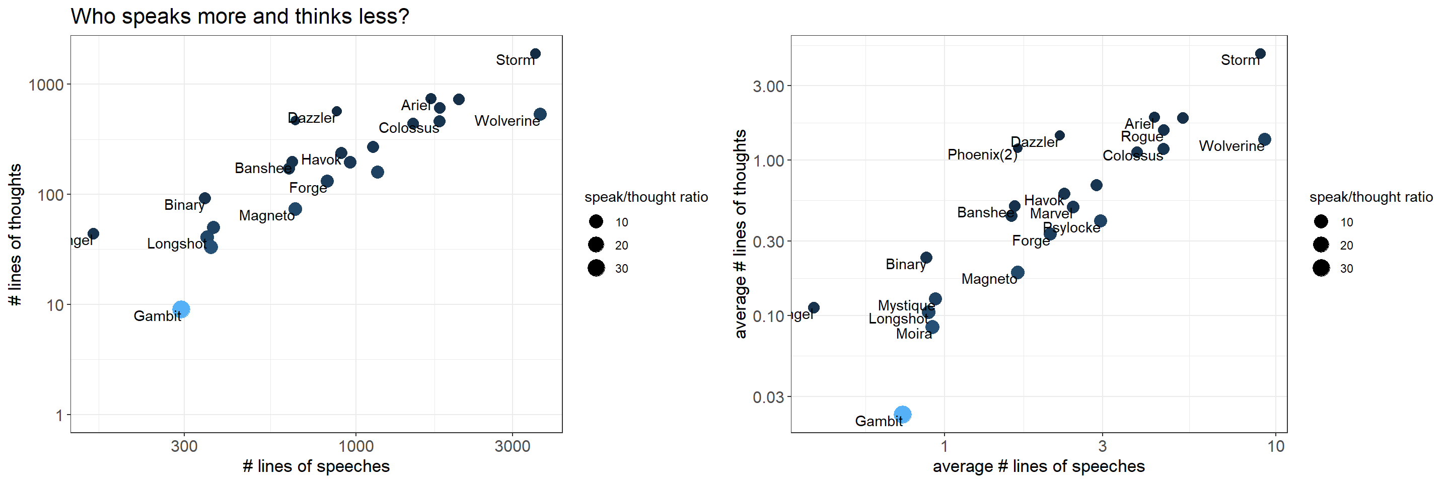
The lollipop plot below is inspired by David Robinson's code. This is my first time making such an intriguing plot!
character_visualization %>%
  group_by(costume, character) %>%
  summarize(total_speech = sum(speech)) %>%
  filter(total_speech > 0) %>%
  ungroup() %>%
  pivot_wider(names_from = "costume", values_from = "total_speech") %>%
  janitor::clean_names() %>%
  mutate(speech_costume_ratio = costume/non_costume,
         character = fct_reorder(character, speech_costume_ratio)) %>%
  ggplot(aes(speech_costume_ratio, character, color = character)) +
  geom_point(size = 4) +
  geom_errorbarh(aes(xmin = 1, xmax = speech_costume_ratio), height = 0, size = 1) +
  scale_x_log10() +
  theme(legend.position = "none") +
  labs(x = "character with and without costume speech ratio",
       y = NULL,
       title = "Lollipop Plot")
Working on characters
Numeric columns visualization:
characters <- characters %>%
  mutate(character = str_remove_all(character, "\\s.+|/.+|\\s?=.+|\\s?,.+|\\(2\\)"))

characters %>%
  select(character, where(is.numeric)) %>%
  pivot_longer(-c(character, issue), names_to = "numeric_column") %>%
  group_by(issue, numeric_column) %>%
  summarize(value = sum(value)) %>%
  ungroup() %>%
  filter(value > 0,
         value < 1e+05) %>%
  mutate(numeric_column = str_replace_all(numeric_column, "_", " ")) %>%
  ggplot(aes(issue, value, color = numeric_column)) +
  geom_line(size = 1) +
  facet_wrap(~numeric_column) +
  theme(legend.position = "none",
        strip.text = element_text(size = 13),
        plot.title = element_text(size = 15)) +
  labs(x = "issue #",
       y = "numeric value summation",
       title = "Numeric columns' summation values")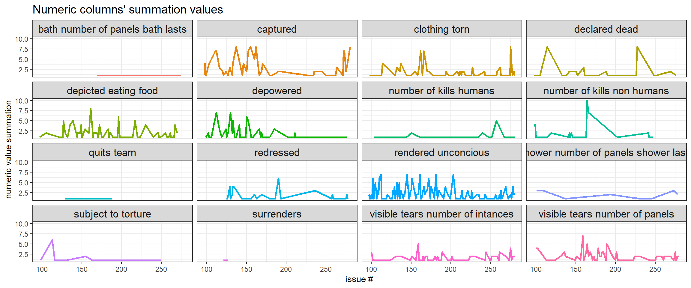
Character graph:
set.seed(2022)
characters %>%
  select(issue, where(is.character)) %>%
  pivot_longer(-c(character, issue), names_to = "character_column") %>%
  drop_na() %>%
  filter(value != "1") %>%
  count(character, value, sort = T) %>%
  head(100) %>%
  ggraph(layout = "fr") +
  geom_edge_link(aes(width = n, color = n), alpha = 0.5) +
  geom_node_point() +
  geom_node_text(aes(label = name, color = name), hjust = 1, vjust = 1, check_overlap = T, size = 5) +
  theme_void() +
  guides(color = "none", edge_color = "none") +
  labs(edge_width = "# of character entanglements",
       title = "How are the characters linked across all issues?")
Working on locations:
locations## # A tibble: 1,413 x 4
## issue location context notes
## <dbl> <chr> <chr> <chr>
## 1 97 Space Dream <NA>
## 2 97 X-Mansion Present <NA>
## 3 97 Rio Diablo Research Facility Present <NA>
## 4 97 Kennedy International Airport Present <NA>
## 5 97 Undisclosed Villain Location Present <NA>
## 6 98 Rockefeller Centre Present <NA>
## 7 98 Boat in the Bahama Out Islands Present <NA>
## 8 98 Sentinel Space Station (former SHIELD Orbital Platform) Present <NA>
## 9 98 X-Mansion Present <NA>
## 10 98 Sentinel Space Station (former SHIELD Orbital Platform) Present <NA>
## # ... with 1,403 more rowsThe popular X-men locations:
locations %>%
  count(location, context, sort = T) %>%
  head(20) %>%
  mutate(location = fct_reorder(location, n, sum)) %>%
  ggplot(aes(n, location, fill = context)) +
  geom_col() +
  labs(x = "#",
       y = "",
       title = "Top 20 locations separated by context")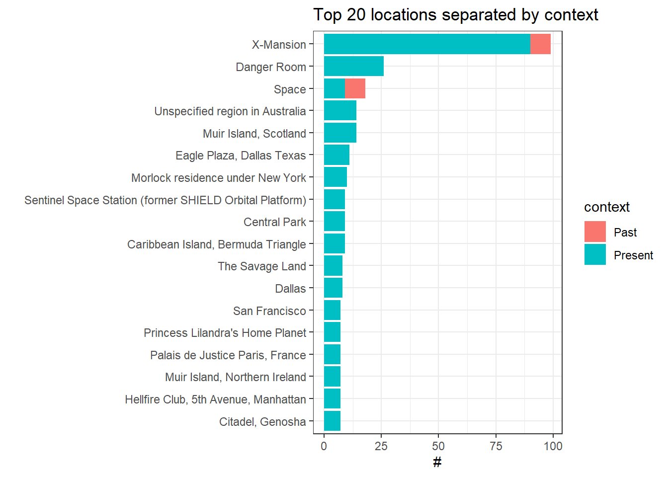
comic_bechdel
comic_bechdel## # A tibble: 308 x 9
## series issue title writer artist cover_artist pass_bechdel page_number notes
## <chr> <dbl> <chr> <chr> <chr> <chr> <chr> <chr> <chr>
## 1 Avenge~ 105 Head~ Steve~ <NA> John Buscema yes 19 <NA>
## 2 Avenge~ 106 A tr~ Steve~ <NA> <NA> no <NA> <NA>
## 3 Avenge~ 107 The ~ Steve~ <NA> <NA> no <NA> <NA>
## 4 Avenge~ 108 Chec~ Steve~ <NA> <NA> no <NA> <NA>
## 5 Avenge~ 109 <NA> Steve~ Don H~ John Buscema no <NA> <NA>
## 6 Avenge~ 110 <NA> Steve~ <NA> Don Heck no <NA> <NA>
## 7 Avenge~ 111 <NA> Steve~ <NA> <NA> no <NA> <NA>
## 8 Avenge~ 112 Plus~ Steve~ <NA> Don Heck yes 4 <NA>
## 9 Avenge~ 113 Your~ Steve~ <NA> <NA> no <NA> <NA>
## 10 Avenge~ 114 The ~ Steve~ <NA> Ron Wilson yes 10 <NA>
## # ... with 298 more rowscomic_bechdel %>%
unnest_tokens(word, title) %>%
anti_join(stop_words) %>%
filter(!is.na(word)) %>%
count(pass_bechdel, word, sort = T) %>%
group_by(pass_bechdel) %>%
slice_max(n, n = 10) %>%
ungroup() %>%
mutate(word = fct_reorder(word, n, sum)) %>%
ggplot(aes(n, word, fill = pass_bechdel)) +
geom_col() +
labs(fill = "bechdel passed?",
y = NULL,
title = "Top 10 words from both bechdel passed and not passed group")
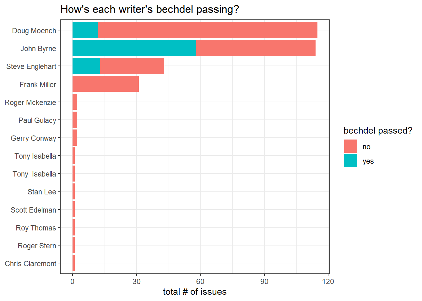
Writers' bechdel passing results:
comic_bechdel %>%
  separate_rows(writer, sep = ", ") %>%
  mutate(writer = str_remove(writer, "\\*")) %>%
  group_by(writer, pass_bechdel) %>%
  summarize(n = n()) %>%
  drop_na() %>%
  ungroup() %>%
  mutate(writer = fct_reorder(writer, n, sum)) %>%
  ggplot(aes(n, writer, fill = pass_bechdel)) +
  geom_col() +
  labs(x = "total # of issues",
       y = NULL,
       fill = "bechdel passed?",
       title = "How's each writer's bechdel passing?")