Penguin Study Data Visualization & Machine Learning by using Tidymodels

Sat, Jan 22, 2022 6-minute read

In this blog post, we will visualize and carry out some machine learning models on the penguin datasets form TidyTuesday.

library(tidyverse)
library(tidymodels)
theme_set(theme_light())

penguins <- readr::read_csv('https://raw.githubusercontent.com/rfordatascience/tidytuesday/master/data/2020/2020-07-28/penguins.csv') %>%
  filter(!is.na(bill_length_mm),
         !is.na(sex)) %>%
  mutate(species = factor(species))

penguins_raw <- readr::read_csv('https://raw.githubusercontent.com/rfordatascience/tidytuesday/master/data/2020/2020-07-28/penguins_raw.csv') %>%
  janitor::clean_names() %>%
  select(-c(stage, region)) %>%
  mutate(species = str_remove(species, "\\s.+"),
         sex = str_to_title(sex))

Penguins' bill:

penguins %>%
  ggplot(aes(bill_length_mm, bill_depth_mm, color = sex)) +
  geom_point(aes(size = flipper_length_mm)) +
  geom_text(aes(label = island), alpha = 0.5, vjust = 1, hjust = 1, check_overlap = T) +
  facet_wrap(~species) +
  scale_size_continuous(range = c(1,5), breaks = c(180, 200, 230)) +
  theme(strip.text = element_text(size = 13),
        plot.title = element_text(size = 16)) +
  labs(x = "bill length (mm)",
       y = "bill depth (mm)",
       color = NULL,
       size = "flipper length (mm)",
       title = "Bill Length & Depth for All 3 Species",
       subtitle = "Text refers to the island where penguins are located")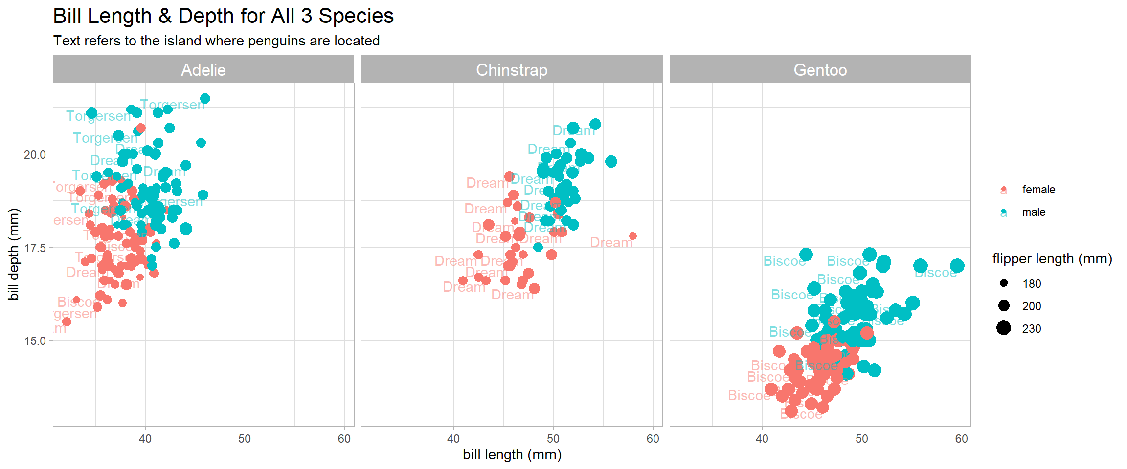

Based on the plot above, it is interesting to find out that Adelie penguins have a deeper bill than their Gentoo counterparts, yet shorter flipper and shorter length.

Penguins' body mass

penguins %>%
  ggplot(aes(sex, body_mass_g, fill = species)) +
  geom_boxplot() +
  facet_wrap(~year) +
  theme(strip.text = element_text(size = 13),
        plot.title = element_text(size = 16)) +
  labs(x = "",
       y = "body mass (g)",
       title = "Yearly Body Mass across All Species")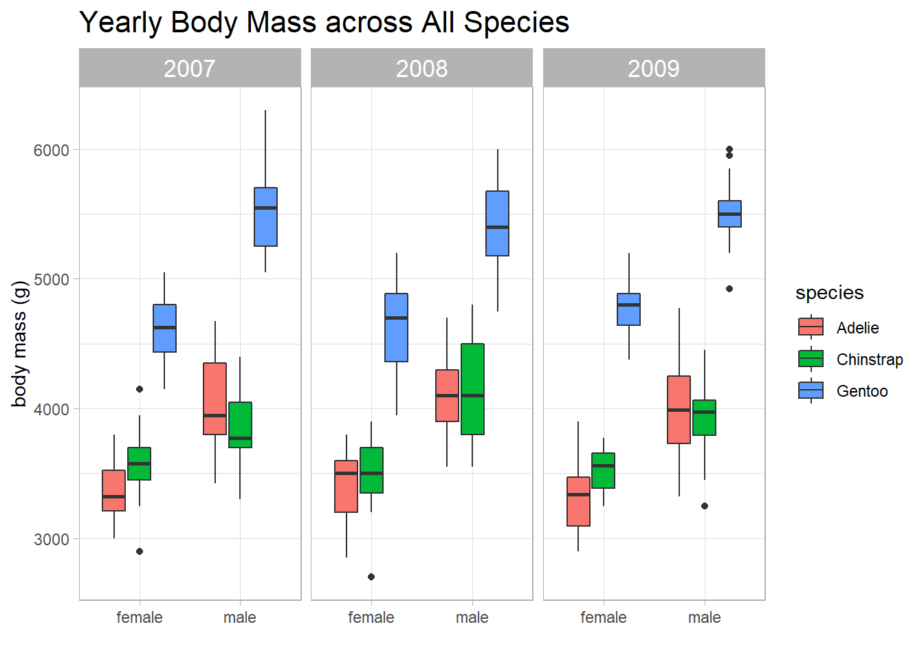

Body index distributions:

penguin_pivot <- penguins %>%
  rename(`bill length (mm)` = bill_length_mm,
         `bill depth (mm)` = bill_depth_mm,
         `flipper length (mm)` = flipper_length_mm,
         `body mass (g)` = body_mass_g) %>%
  pivot_longer(c(3:6), names_to = "variable") 
  

penguin_pivot %>%
 ggplot(aes(value, fill = sex)) +
  geom_histogram(alpha = 0.7) +
  facet_wrap(~variable, scales = "free") +
  labs(x = "respective body value",
       fill = NULL,
       title = "How Are Penguins' Body Indexes Distributed?") +
  theme(strip.text = element_text(size = 13),
        plot.title = element_text(size = 16))

Machine Learning:

I normally use the caret package to do my machine learning work, but now I am transferring to using tidymodels, as it does provide a coherent ecosystem as tidyverse provides. Since I am learning how to use tidymodels, this dataset is a great way to get more familiarity on how to use it. This machine learning section is inspired by Julia Silge's code and David Robinson's code. Many functions built inside the meta-package are my first time using them. Another note here is some code might be identical to the links provided above, with some slight modification.

I. Predicting the penguins' sex

#split up the data into training and testing data by using initial_split()
set.seed(2022)
penguin_split <- initial_split(penguins, prop = 0.8, strata = sex)
penguin_training <- training(penguin_split)
penguin_testing <- testing(penguin_split)

training_splits <- penguin_training %>%
  vfold_cv(10)

# logistic regression
glm_set <- logistic_reg() %>%
  set_engine("glm") 

# random forest classification
rf_set <- rand_forest() %>%
  set_engine("ranger") %>%
  set_mode("classification")

# define a work flow
penguin_wf <- workflow() %>%
  add_formula(factor(sex) ~ bill_length_mm + bill_depth_mm + flipper_length_mm + body_mass_g)

# add models here
glm_rs <- penguin_wf %>%
  add_model(glm_set) %>%
  fit_resamples(training_splits,
                control = control_resamples(save_pred = TRUE)) 

rf_rs <- penguin_wf %>%
  add_model(rf_set) %>%
  fit_resamples(training_splits,
                control = control_resamples(save_pred = TRUE)) 

collect_metrics(rf_rs)

## # A tibble: 2 x 6
##   .metric  .estimator  mean     n std_err .config             
##   <chr>    <chr>      <dbl> <int>   <dbl> <chr>               
## 1 accuracy binary     0.895    10  0.0157 Preprocessor1_Model1
## 2 roc_auc  binary     0.951    10  0.0152 Preprocessor1_Model1

Model evaluations:

collect_metrics(glm_rs)

## # A tibble: 2 x 6
##   .metric  .estimator  mean     n std_err .config             
##   <chr>    <chr>      <dbl> <int>   <dbl> <chr>               
## 1 accuracy binary     0.895    10  0.0155 Preprocessor1_Model1
## 2 roc_auc  binary     0.955    10  0.0126 Preprocessor1_Model1

collect_metrics(rf_rs)

## # A tibble: 2 x 6
##   .metric  .estimator  mean     n std_err .config             
##   <chr>    <chr>      <dbl> <int>   <dbl> <chr>               
## 1 accuracy binary     0.895    10  0.0157 Preprocessor1_Model1
## 2 roc_auc  binary     0.951    10  0.0152 Preprocessor1_Model1

It looks like the linear model has a slightly better fitting than its random forest counterpart.

Confusion Matrix:

glm_rs %>%
  conf_mat_resampled()

## # A tibble: 4 x 3
##   Prediction Truth   Freq
##   <fct>      <fct>  <dbl>
## 1 female     female  11.5
## 2 female     male     1.1
## 3 male       female   1.7
## 4 male       male    12.3

rf_rs %>%
  conf_mat_resampled()

## # A tibble: 4 x 3
##   Prediction Truth   Freq
##   <fct>      <fct>  <dbl>
## 1 female     female  11.8
## 2 female     male     1.4
## 3 male       female   1.4
## 4 male       male    12

glm_rs %>%
  collect_predictions() %>%
  rename(sex = `factor(sex)`) %>%
  group_by(id) %>%
  roc_curve(sex, .pred_female) %>%
  ggplot(aes(1 - specificity, sensitivity, color = id)) +
  geom_abline(lty = 2, size = 1.5) +
  geom_path(show.legend = FALSE, alpha = 0.6, size = 1) +
  coord_fixed(ratio = 1) +
  labs(title = "The ROC Curves for All 10 Folds")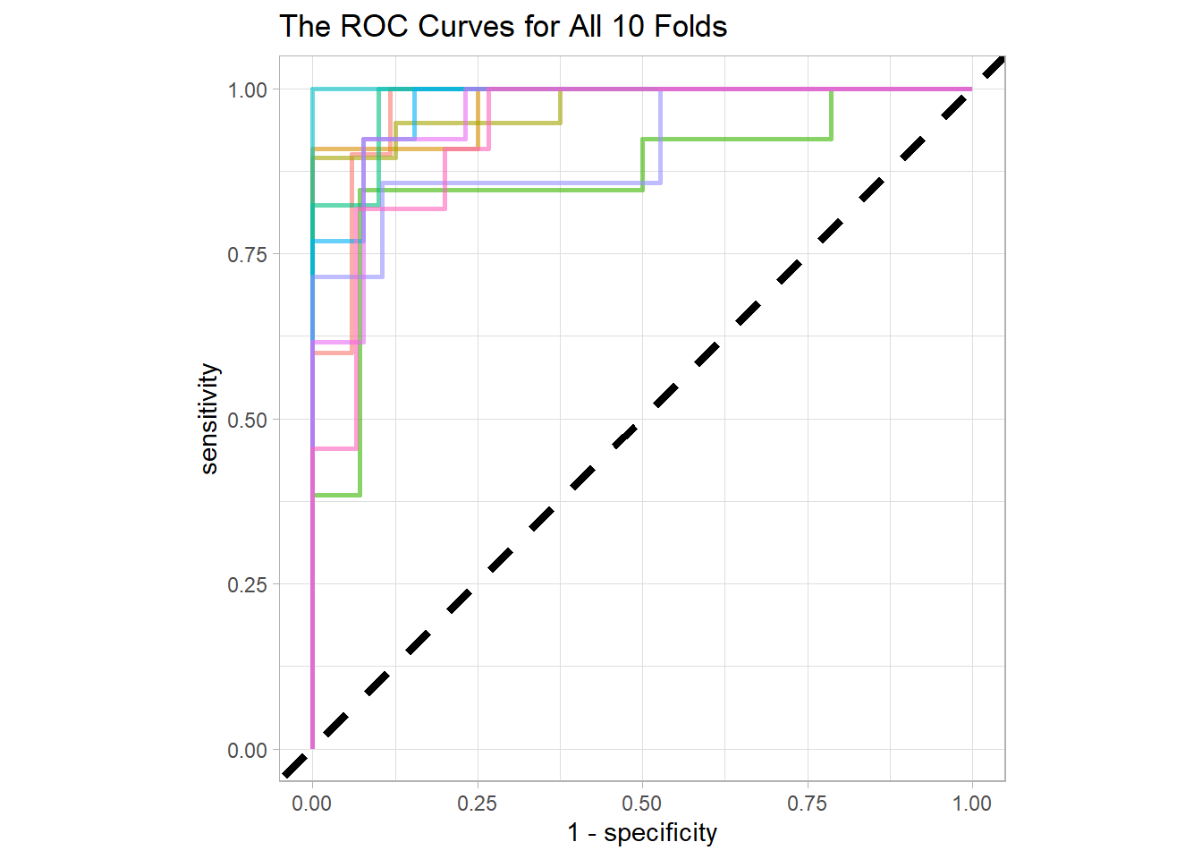

Final Model

penguin_final <- penguin_wf %>%
  add_model(glm_set) %>%
  last_fit(penguin_split) 

penguin_final %>%
  unnest(.predictions) %>%
  rename(sex = 9) %>%
  conf_mat(sex, .pred_class)

##           Truth
## Prediction female male
##     female     31    3
##     male        2   31

penguin_final$.workflow[[1]] %>%
  tidy(exponentiate = T)

## # A tibble: 5 x 5
##   term              estimate std.error statistic  p.value
##   <chr>                <dbl>     <dbl>     <dbl>    <dbl>
## 1 (Intercept)       1.81e-24  9.06        -6.03  1.62e- 9
## 2 bill_length_mm    1.12e+ 0  0.0514       2.14  3.21e- 2
## 3 bill_depth_mm     7.27e+ 0  0.265        7.48  7.62e-14
## 4 flipper_length_mm 9.69e- 1  0.0389      -0.809 4.18e- 1
## 5 body_mass_g       1.01e+ 0  0.000903     5.87  4.43e- 9

II. Predicting penguins' species

penguin_wf2 <- workflow() %>%
  add_formula(species ~ bill_length_mm + bill_depth_mm + flipper_length_mm + body_mass_g)

species_model <- penguin_wf2 %>%
  add_model(rf_set) %>%
  fit_resamples(training_splits,
                metrics = metric_set(accuracy, kap, roc_auc),
                control = control_resamples(save_pred = TRUE)) 

species_model %>%
  collect_metrics()

## # A tibble: 3 x 6
##   .metric  .estimator  mean     n std_err .config             
##   <chr>    <chr>      <dbl> <int>   <dbl> <chr>               
## 1 accuracy multiclass 0.970    10 0.0121  Preprocessor1_Model1
## 2 kap      multiclass 0.954    10 0.0184  Preprocessor1_Model1
## 3 roc_auc  hand_till  0.999    10 0.00116 Preprocessor1_Model1

penguin_wf2 %>%
  add_model(rf_set) %>%
  last_fit(penguin_split) %>%
  unnest(.predictions) %>%
  conf_mat(species, .pred_class)

##            Truth
## Prediction  Adelie Chinstrap Gentoo
##   Adelie        29         2      0
##   Chinstrap      1        10      0
##   Gentoo         0         0     25

All models above perform fantastically well, in part due to the small size of the dataset and the easy prediction.

Working on penguins_raw

penguins_raw <- penguins_raw %>%
  rename(delta_15 = delta_15_n_o_oo,
         delta_13 = delta_13_c_o_oo)

penguins_raw %>%
  count(delta_13, sort = T)

## # A tibble: 332 x 2
##    delta_13     n
##       <dbl> <int>
##  1     NA      13
##  2    -27.0     1
##  3    -27.0     1
##  4    -26.9     1
##  5    -26.9     1
##  6    -26.9     1
##  7    -26.9     1
##  8    -26.8     1
##  9    -26.8     1
## 10    -26.8     1
## # ... with 322 more rows

penguins_raw %>%
  ggplot(aes(delta_13, delta_15, color = sex, size = body_mass_g, shape = species)) +
  geom_point(alpha = 0.8) +
  labs(x = "Delta 13",
       y = "Delta 15",
       size = "body mass (g)",
       title = "The Relations betweeen delta 13 and 15 across All Species and Sexes",
       subtitle = "Delta 13 and 15 are the measurements of dietary comparison") +
  theme(plot.title = element_text(size = 16))

The heavier of penguins are, the less Delta 15 and 13 their measurements are for both male and female penguins for Adelie and Gentoo species in particular.

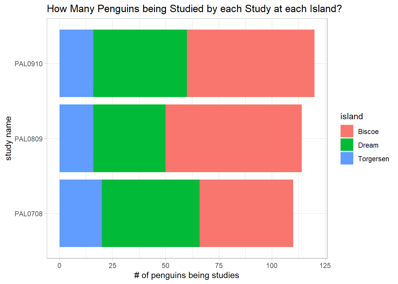
penguins_raw %>% 
  count(study_name, island, sort = T) %>%
  ggplot(aes(n, study_name, fill = island)) +
  geom_col() +
  labs(x = "# of penguins being studies",
       y = "study name",
       title = "How Many Penguins being Studied by each Study at each Island?")