Extinct Plants Data Visualization
In this blog post, we will analyze extinct plants. The datasets are from TidyTuesday, where you can find them here.
library(tidyverse)
library(widyr)
library(ggraph)
theme_set(theme_light())
plants <- read_csv('https://raw.githubusercontent.com/rfordatascience/tidytuesday/master/data/2020/2020-08-18/plants.csv') %>%
separate(binomial_name, sep = " ", into = c("genus", "species")) %>%
mutate(species = str_to_title(species))
actions <- read_csv('https://raw.githubusercontent.com/rfordatascience/tidytuesday/master/data/2020/2020-08-18/actions.csv')
threats <- read_csv('https://raw.githubusercontent.com/rfordatascience/tidytuesday/master/data/2020/2020-08-18/threats.csv') %>%
separate(binomial_name, sep = " ", into = c("genus", "species")) %>%
mutate(species = str_to_title(species))When did plants disappear?
plants %>%
  mutate(year_last_seen = str_remove_all(year_last_seen, "^.*-|^.*\\s")) %>%
  count(continent, year_last_seen, sort = T) %>%
  filter(!is.na(year_last_seen)) %>%
  ggplot(aes(year_last_seen, n, fill = continent)) +
  geom_col(aes(group = continent)) +
  labs(x = "year last seen",
       y = "distinct plant count",
       fill = NULL,
       title = "When Did the Plants Go Extinct?")
Data wrangling:
- Threats
plant_threats <- plants %>%
  select(!contains("action")) %>%
  pivot_longer(cols = contains("threat"), names_to = "threat") %>%
  #filter(value == 1) %>%
  mutate(threat = str_remove(threat, "^.+_"))

plant_threats
## # A tibble: 6,000 x 9
## genus species country continent group year_last_seen red_list_catego~ threat
## <chr> <chr> <chr> <chr> <chr> <chr> <chr> <chr>
## 1 Abuti~ Pitcai~ Pitcai~ Oceania Flow~ 2000-2020 Extinct in the ~ AA
## 2 Abuti~ Pitcai~ Pitcai~ Oceania Flow~ 2000-2020 Extinct in the ~ BRU
## 3 Abuti~ Pitcai~ Pitcai~ Oceania Flow~ 2000-2020 Extinct in the ~ RCD
## 4 Abuti~ Pitcai~ Pitcai~ Oceania Flow~ 2000-2020 Extinct in the ~ ISGD
## 5 Abuti~ Pitcai~ Pitcai~ Oceania Flow~ 2000-2020 Extinct in the ~ EPM
## 6 Abuti~ Pitcai~ Pitcai~ Oceania Flow~ 2000-2020 Extinct in the ~ CC
## 7 Abuti~ Pitcai~ Pitcai~ Oceania Flow~ 2000-2020 Extinct in the ~ HID
## 8 Abuti~ Pitcai~ Pitcai~ Oceania Flow~ 2000-2020 Extinct in the ~ P
## 9 Abuti~ Pitcai~ Pitcai~ Oceania Flow~ 2000-2020 Extinct in the ~ TS
## 10 Abuti~ Pitcai~ Pitcai~ Oceania Flow~ 2000-2020 Extinct in the ~ NSM
## # ... with 5,990 more rows, and 1 more variable: value <dbl>plant_threats has the threat column, a threat code shortcut. In order to get the full threat name, we need to do a bit more work to obtain threat_type_crosswalk:
threat_type_crosswalk <- threats %>%
  bind_cols(plant_threats %>% select(threat)) %>%
  select(threat_type, threat) %>%
  distinct()

threat_type_crosswalk
## # A tibble: 12 x 2
## threat_type threat
## <chr> <chr>
## 1 Agriculture & Aquaculture AA
## 2 Biological Resource Use BRU
## 3 Commercial Development RCD
## 4 Invasive Species ISGD
## 5 Energy Production & Mining EPM
## 6 Climate Change CC
## 7 Human Intrusions HID
## 8 Pollution P
## 9 Transportation Corridor TS
## 10 Natural System Modifications NSM
## 11 Geological Events GE
## 12 Unknown NANow join them together for full information:
threat_joined <- plant_threats %>%
  left_join(threat_type_crosswalk, by = "threat") %>%
  filter(value == 1)

threat_joined %>%
  count(continent, threat_type, sort = T) %>%
  ggplot(aes(continent, threat_type, fill = n)) +
  geom_tile() +
  scale_fill_gradient(high = "red",
                      low = "green") +
  theme(axis.text.x = element_text(angle = 90),
        panel.grid = element_blank()) +
  labs(x = NULL,
       y = NULL,
       fill = "#",
       title = "What is the Relation between Threat Type and Continent?")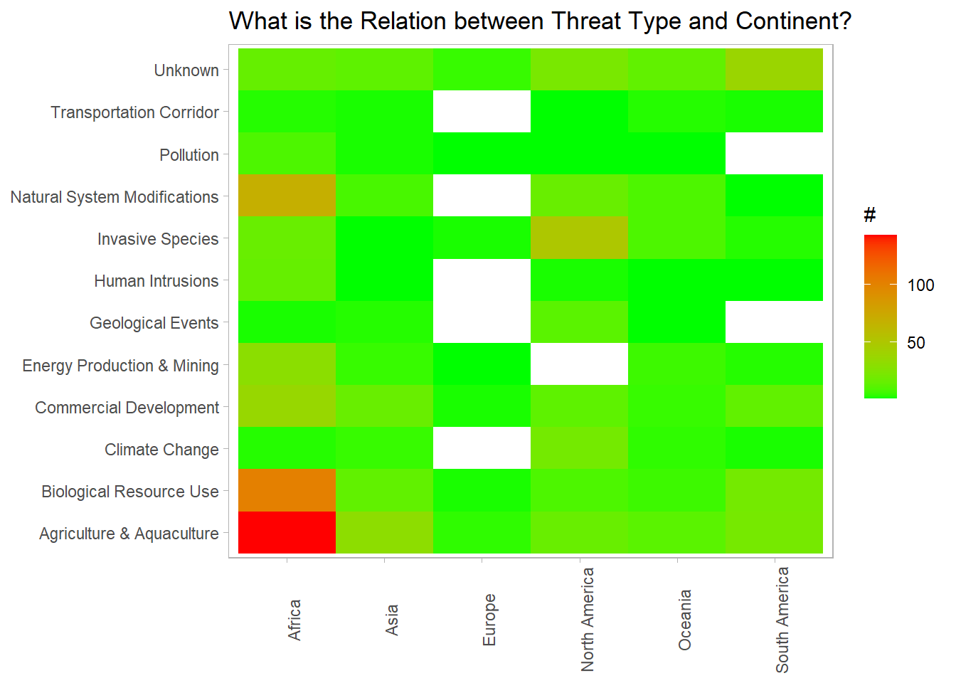
Clearly, African plants suffer the “Agriculture & Aquaculture” type threat, and then the “Biological Resource Use” one from the heatmap above.
Correlation graph:
set.seed(2022)

threat_joined %>%
  count(species, continent) %>%
  pairwise_cor(species, continent, n, sort = T) %>%
  head(1000) %>%
  ggraph(layout = "fr") +
  geom_edge_link(aes(color = correlation), alpha = 0.5) +
  geom_node_point() +
  geom_node_text(aes(label = name), hjust = 1, vjust = 1, check_overlap = T, size = 5) +
  theme_void() +
  guides(color = "none", edge_color = "none") +
  labs(edge_color = "correlation",
       title = "How are species correlated?") +
  theme(plot.title = element_text(size = 18))
4 clusters of species!
- Actions
plant_actions <- plants %>%
  select(!contains("threat")) %>%
  pivot_longer(cols = contains("action"), names_to = "action") %>%
  #filter(value == 1) %>%
  mutate(action = str_remove(action, "^.+_"))

plant_actions
## # A tibble: 3,000 x 9
## genus species country continent group year_last_seen red_list_catego~ action
## <chr> <chr> <chr> <chr> <chr> <chr> <chr> <chr>
## 1 Abuti~ Pitcai~ Pitcai~ Oceania Flow~ 2000-2020 Extinct in the ~ LWP
## 2 Abuti~ Pitcai~ Pitcai~ Oceania Flow~ 2000-2020 Extinct in the ~ SM
## 3 Abuti~ Pitcai~ Pitcai~ Oceania Flow~ 2000-2020 Extinct in the ~ LP
## 4 Abuti~ Pitcai~ Pitcai~ Oceania Flow~ 2000-2020 Extinct in the ~ RM
## 5 Abuti~ Pitcai~ Pitcai~ Oceania Flow~ 2000-2020 Extinct in the ~ EA
## 6 Abuti~ Pitcai~ Pitcai~ Oceania Flow~ 2000-2020 Extinct in the ~ NA
## 7 Acaena Exigua United~ North Am~ Flow~ 1980-1999 Extinct LWP
## 8 Acaena Exigua United~ North Am~ Flow~ 1980-1999 Extinct SM
## 9 Acaena Exigua United~ North Am~ Flow~ 1980-1999 Extinct LP
## 10 Acaena Exigua United~ North Am~ Flow~ 1980-1999 Extinct RM
## # ... with 2,990 more rows, and 1 more variable: value <dbl>Just like threat_type_crosswalk, here is action_type_crosswalk:
action_type_crosswalk <- actions %>%
  bind_cols(plant_actions %>% select(action)) %>%
  select(action_type, action) %>%
  distinct()

action_type_crosswalk
## # A tibble: 6 x 2
## action_type action
## <chr> <chr>
## 1 Land & Water Protection LWP
## 2 Species Management SM
## 3 Law & Policy LP
## 4 Research & Monitoring RM
## 5 Education & Awareness EA
## 6 Unknown NAaction_joined <- plant_actions %>%
left_join(action_type_crosswalk, by = "action") %>%
filter(value == 1) %>%
select(-c(action, value))
action_joined## # A tibble: 559 x 8
## genus species country continent group year_last_seen red_list_catego~
## <chr> <chr> <chr> <chr> <chr> <chr> <chr>
## 1 Abutilon Pitcairn~ Pitcai~ Oceania Flow~ 2000-2020 Extinct in the ~
## 2 Abutilon Pitcairn~ Pitcai~ Oceania Flow~ 2000-2020 Extinct in the ~
## 3 Abutilon Pitcairn~ Pitcai~ Oceania Flow~ 2000-2020 Extinct in the ~
## 4 Acaena Exigua United~ North Am~ Flow~ 1980-1999 Extinct
## 5 Acalypha Dikuluwe~ Congo Africa Flow~ 1940-1959 Extinct
## 6 Acalypha Rubriner~ Saint ~ Africa Flow~ Before 1900 Extinct
## 7 Acalypha Wilderi Cook I~ Oceania Flow~ 1920-1939 Extinct
## 8 Acer Hilaense China Asia Flow~ 1920-1939 Extinct in the ~
## 9 Achyranthes Atollens~ United~ North Am~ Flow~ 1960-1979 Extinct
## 10 Adenophorus Periens United~ North Am~ Fern~ 2000-2020 Extinct
## # ... with 549 more rows, and 1 more variable: action_type <chr>action_joined %>%
count(continent, action_type, sort = T) %>%
filter(action_type != "Unknown") %>%
mutate(action_type = fct_reorder(action_type, n, sum),
continent = fct_reorder(continent, n, sum)) %>%
ggplot(aes(n, action_type, fill = continent)) +
geom_col() +
labs(y = "action type",
fill = NULL)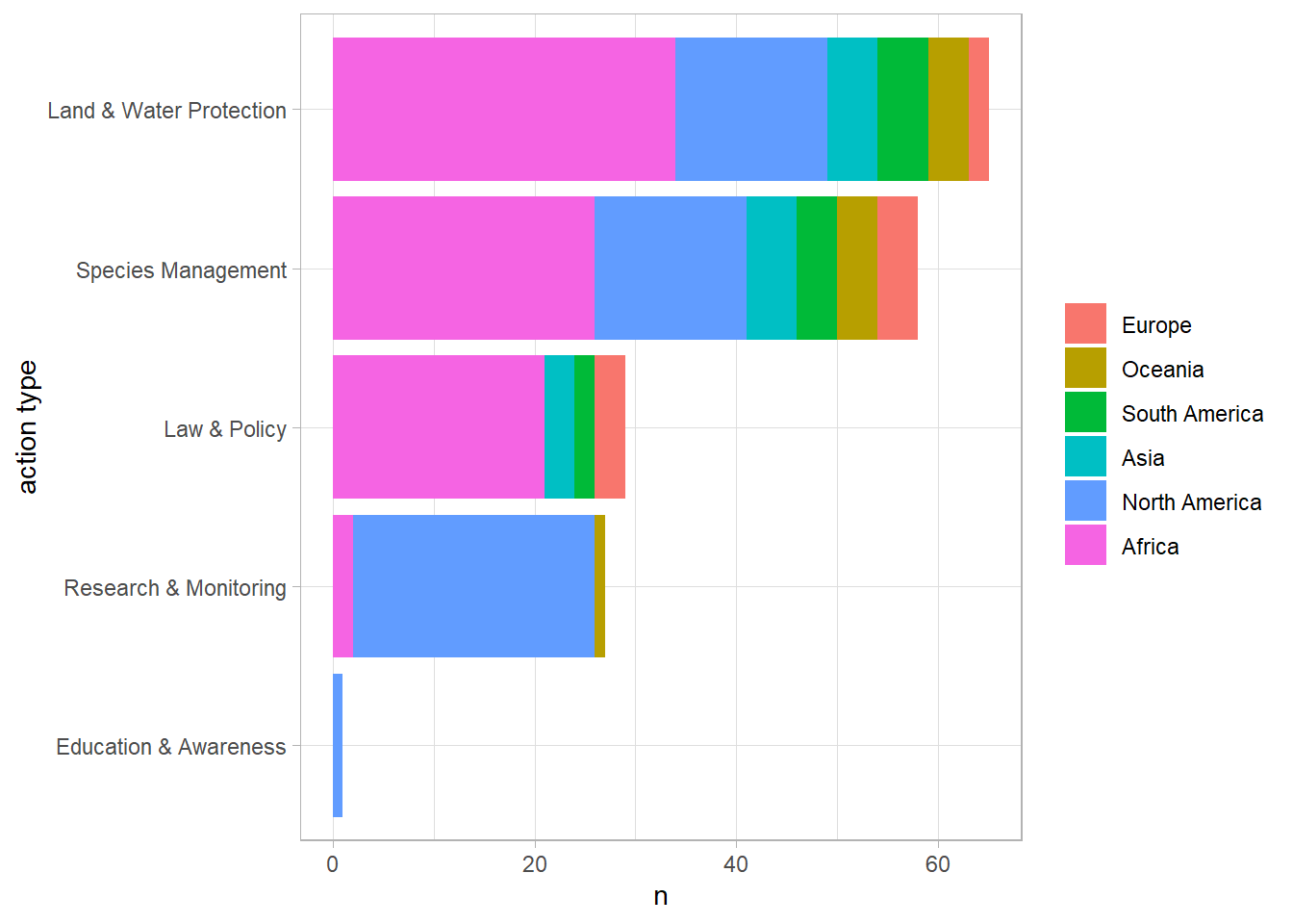
Land & Water Protection is the most acted type overall and surprisingly North America is the only continent that has acted Education & Awareness.