Chopped Data Visualization

In this blog post, I will analyze a dataset about the TV show Chopped. Nothing do I know about the show, but this is a great opportunity to dive into a dataset that I do not know any background information. Let’s see what we can find from it. Here is the source of data (link).

library(tidyverse)
library(lubridate)
library(tidytext)
library(widyr)
library(ggraph)
theme_set(theme_light())

chopped <- read_tsv('https://raw.githubusercontent.com/rfordatascience/tidytuesday/master/data/2020/2020-08-25/chopped.tsv') %>%
  mutate(air_date = mdy(air_date)) %>%
  filter(episode_rating > 6)

chopped

## # A tibble: 463 x 21
##    season season_episode series_episode episode_rating episode_name             
##     <dbl>          <dbl>          <dbl>          <dbl> <chr>                    
##  1      1              1              1            9.2 Octopus, Duck, Animal Cr~
##  2      1              2              2            8.8 Tofu, Blueberries, Oyste~
##  3      1              3              3            8.9 Avocado, Tahini, Bran Fl~
##  4      1              4              4            8.5 Banana, Collard Greens, ~
##  5      1              5              5            8.8 Yucca, Watermelon, Torti~
##  6      1              6              6            8.5 Canned Peaches, Rice Cak~
##  7      1              7              7            8.8 Quail, Arctic Char, Beer 
##  8      1              8              8            9   Coconut, Calamari, Donuts
##  9      1              9              9            8.9 Mac & Cheese, Cola, Bacon
## 10      1             10             10            8.8 String Cheese, Jicama, G~
## # ... with 453 more rows, and 16 more variables: episode_notes <chr>,
## #   air_date <date>, judge1 <chr>, judge2 <chr>, judge3 <chr>, appetizer <chr>,
## #   entree <chr>, dessert <chr>, contestant1 <chr>, contestant1_info <chr>,
## #   contestant2 <chr>, contestant2_info <chr>, contestant3 <chr>,
## #   contestant3_info <chr>, contestant4 <chr>, contestant4_info <chr>

chopped %>%
  ggplot(aes(air_date, episode_rating)) +
  geom_point(aes(color = factor(season)), 
             show.legend = F,
             size = 2) +
  geom_smooth(method = "loess",
              se = F,
              size = 2) +
  scale_x_date(date_breaks = "6 months",
               date_labels = "%Y-%m") +
  labs(x = "air date",
       y = "episode rating",
       title = "Episode Ratings with the Air Date",
       subtitle = "Colors represent the season")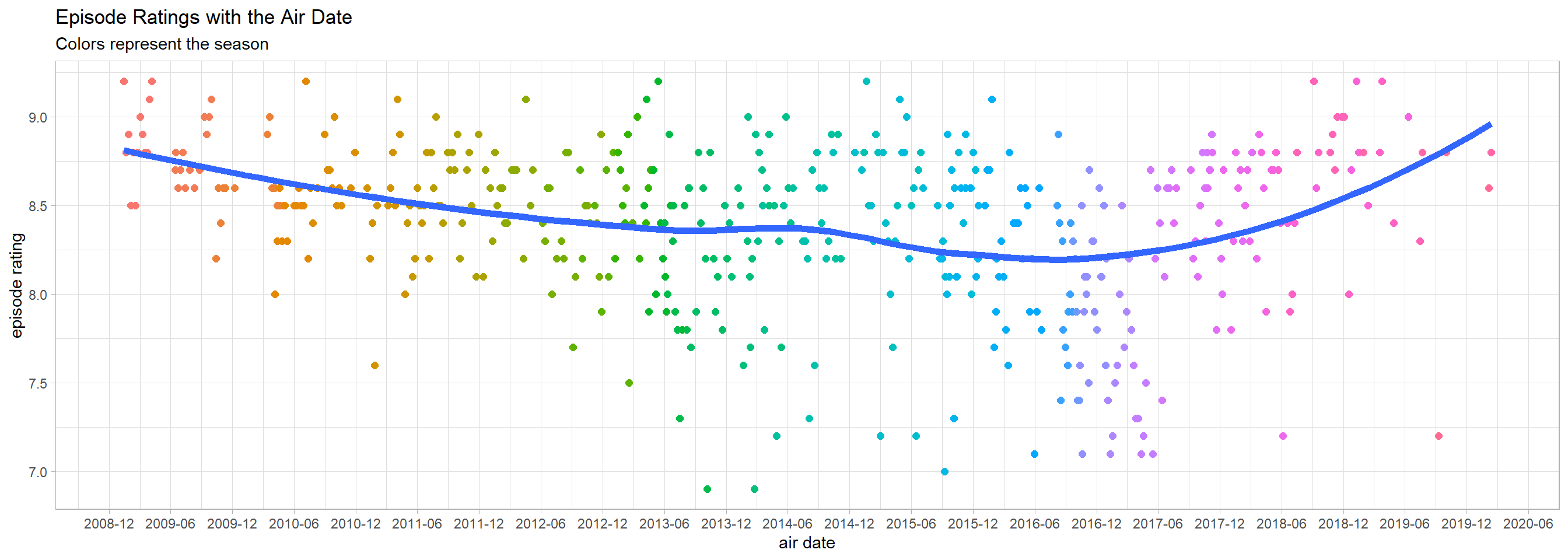

It seems like the overall episode rating stayed roughly the same all the time, although there was a little dip in the middle somewhere.

chopped %>%
  ggplot(aes(episode_rating)) +
  geom_histogram(binwidth = 0.1)

Some ideas in this blog post are inspired by David Robinson’s code.

ingredients <- chopped %>%
  select(season, season_episode, episode_rating, appetizer:dessert) %>%
  pivot_longer(cols = c(appetizer:dessert), names_to = "course", values_to = "ingredient") %>%
  separate_rows(ingredient, sep = ",\\s") %>%
  mutate(course = factor(course, levels = c("appetizer", "entree", "dessert")))

Popular ingredients:

ingredients %>%
  count(course, ingredient, sort = T) %>%
  group_by(course) %>%
  slice_max(n, n = 20) %>%
  ungroup() %>%
  mutate(ingredient = reorder_within(ingredient, n, course)) %>%
  ggplot(aes(n, ingredient, fill = ingredient)) +
  geom_col(show.legend = F) +
  scale_y_reordered() +
  facet_wrap(~course, scales = "free_y") +
  labs(x = "# of times ingredient appears",
       y = NULL,
       title = "Which are the most popular ingredients?")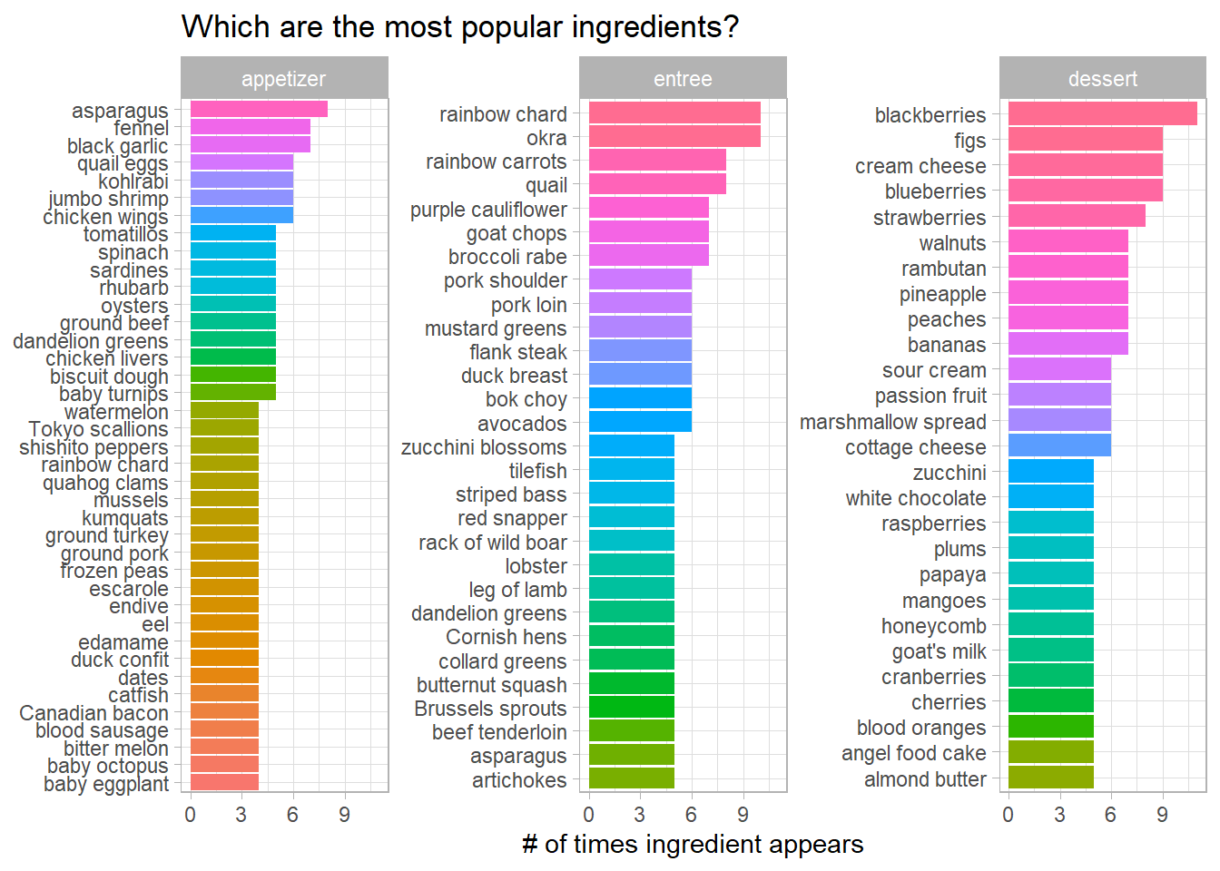

How ingredients are correlated within each season?

set.seed(2022)

ingredients %>%
  add_count(ingredient) %>%
  filter(n > 10) %>%
  pairwise_cor(ingredient, season, sort = T) %>%
  head(100) %>%
  ggraph(layout = "fr") +
  geom_edge_link(aes(color = correlation, width = correlation), alpha = 0.5) +
  geom_node_point() +
  geom_node_text(aes(label = name), hjust = 1, vjust = 1, check_overlap = T, size = 5) +
  theme_void() +
  guides(color = "none", edge_color = "none") +
  labs(edge_color = "correlation",
       title = "How are ingredients correlated within each season?") +
  theme(plot.title = element_text(size = 18))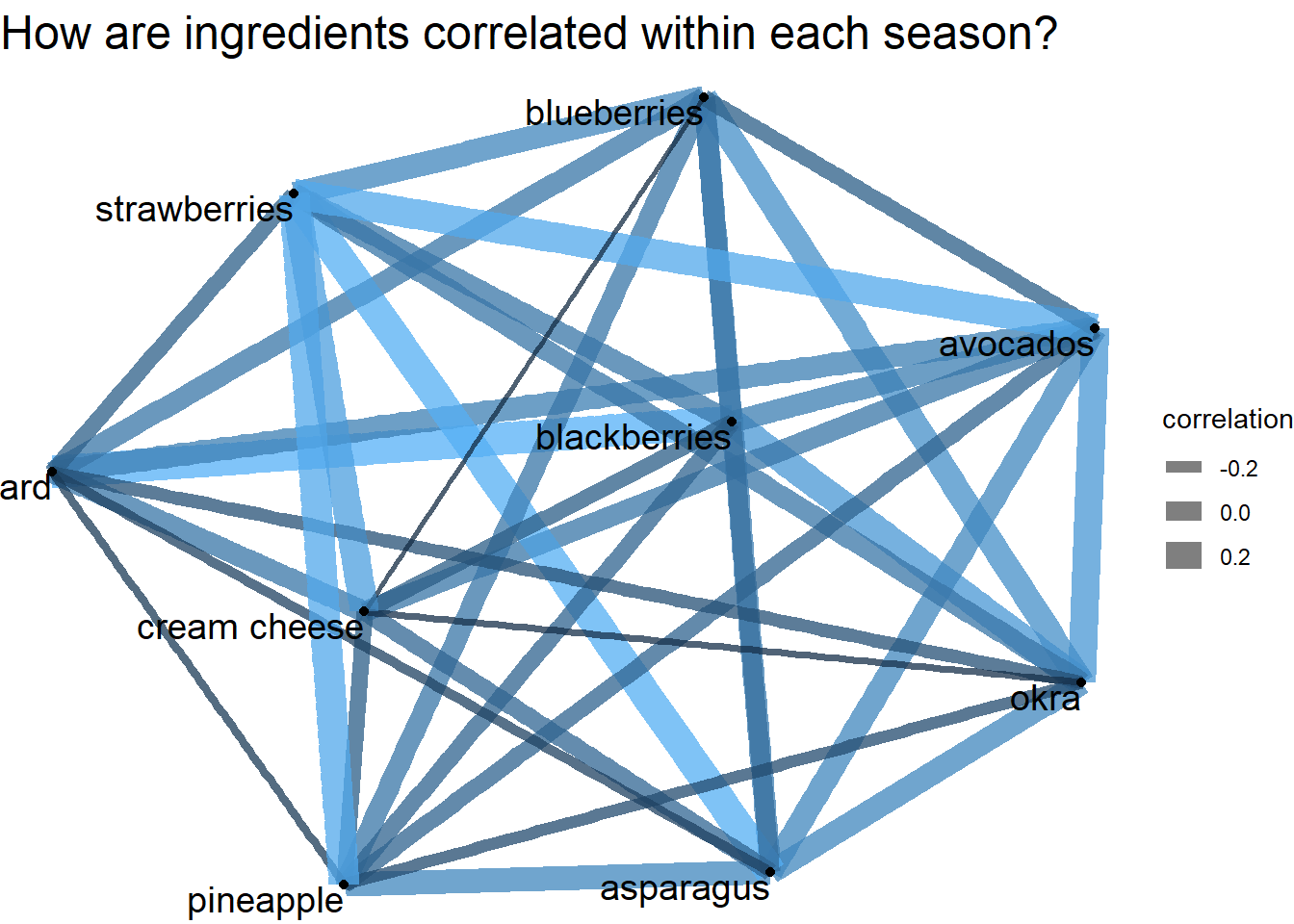

new_ingredients <- ingredients %>%
  add_count(ingredient) %>%
  filter(n > 5) %>%
  group_by(ingredient) %>%
  summarize(first_season = min(season),
            avg_season = mean(season),
            last_season = max(season)) %>%
  slice(c(1:7), tail(row_number(), n = 7))

ingredients %>%
  semi_join(new_ingredients, by = "ingredient") %>%
  mutate(ingredient = fct_reorder(ingredient, season, median)) %>%
  ggplot(aes(season, ingredient, fill = ingredient)) +
  geom_boxplot(show.legend = F)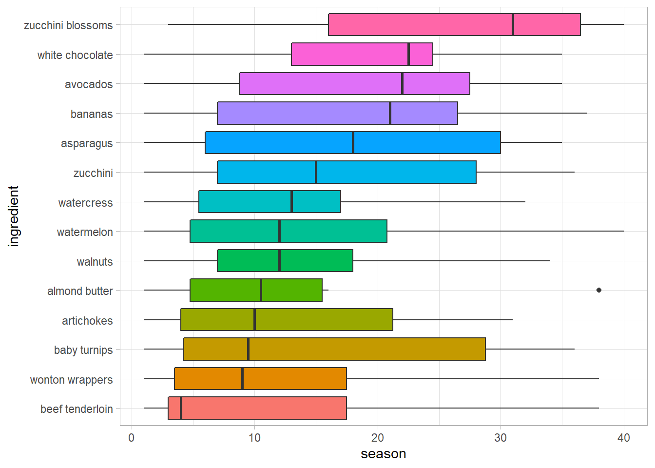

Interestingly, almond butter was used in the first 15 seasons or so, but then it was abandoned until almost the Season 39.