Global Crop Yields Data Processing & Visualization
This blog post analyzes data about the global crop yields from TidyTuesday. The primary focus of this data processing/visualization is between 1961 to 2020.
library(tidyverse)
library(countrycode)
theme_set(theme_light())
key_crop_yields <- read_csv('https://raw.githubusercontent.com/rfordatascience/tidytuesday/master/data/2020/2020-09-01/key_crop_yields.csv')
fertilizer <- read_csv('https://raw.githubusercontent.com/rfordatascience/tidytuesday/master/data/2020/2020-09-01/cereal_crop_yield_vs_fertilizer_application.csv')
tractors <- read_csv('https://raw.githubusercontent.com/rfordatascience/tidytuesday/master/data/2020/2020-09-01/cereal_yields_vs_tractor_inputs_in_agriculture.csv')
land_use <- read_csv('https://raw.githubusercontent.com/rfordatascience/tidytuesday/master/data/2020/2020-09-01/land_use_vs_yield_change_in_cereal_production.csv')
arable_land <- read_csv('https://raw.githubusercontent.com/rfordatascience/tidytuesday/master/data/2020/2020-09-01/arable_land_pin.csv')Working on key_crop_yields:
key_crop_yields## # A tibble: 13,075 x 14
## Entity Code Year `Wheat (tonnes pe~` `Rice (tonnes ~` `Maize (tonnes~`
## <chr> <chr> <dbl> <dbl> <dbl> <dbl>
## 1 Afghanistan AFG 1961 1.02 1.52 1.4
## 2 Afghanistan AFG 1962 0.974 1.52 1.4
## 3 Afghanistan AFG 1963 0.832 1.52 1.43
## 4 Afghanistan AFG 1964 0.951 1.73 1.43
## 5 Afghanistan AFG 1965 0.972 1.73 1.44
## 6 Afghanistan AFG 1966 0.867 1.52 1.44
## 7 Afghanistan AFG 1967 1.12 1.92 1.41
## 8 Afghanistan AFG 1968 1.16 1.95 1.71
## 9 Afghanistan AFG 1969 1.19 1.98 1.72
## 10 Afghanistan AFG 1970 0.956 1.81 1.48
## # ... with 13,065 more rows, and 8 more variables:
## # `Soybeans (tonnes per hectare)` <dbl>,
## # `Potatoes (tonnes per hectare)` <dbl>, `Beans (tonnes per hectare)` <dbl>,
## # `Peas (tonnes per hectare)` <dbl>, `Cassava (tonnes per hectare)` <dbl>,
## # `Barley (tonnes per hectare)` <dbl>,
## # `Cocoa beans (tonnes per hectare)` <dbl>,
## # `Bananas (tonnes per hectare)` <dbl>Most of the column names of the tibble are long and not in a neat form. There are two ways to clean this up:
- using
reanme_within conjunction withstr_remove_all()
key_crop_yields %>%
  janitor::clean_names() %>%
  rename_with(.cols = c(3:14), .fn = ~ str_remove_all(., "_.+$"))
## # A tibble: 13,075 x 14
## entity code year wheat rice maize soybeans potatoes beans peas cassava
## <chr> <chr> <dbl> <dbl> <dbl> <dbl> <dbl> <dbl> <dbl> <dbl> <dbl>
## 1 Afghanis~ AFG 1961 1.02 1.52 1.4 NA 8.67 NA NA NA
## 2 Afghanis~ AFG 1962 0.974 1.52 1.4 NA 7.67 NA NA NA
## 3 Afghanis~ AFG 1963 0.832 1.52 1.43 NA 8.13 NA NA NA
## 4 Afghanis~ AFG 1964 0.951 1.73 1.43 NA 8.6 NA NA NA
## 5 Afghanis~ AFG 1965 0.972 1.73 1.44 NA 8.8 NA NA NA
## 6 Afghanis~ AFG 1966 0.867 1.52 1.44 NA 9.07 NA NA NA
## 7 Afghanis~ AFG 1967 1.12 1.92 1.41 NA 9.8 NA NA NA
## 8 Afghanis~ AFG 1968 1.16 1.95 1.71 NA 10 NA NA NA
## 9 Afghanis~ AFG 1969 1.19 1.98 1.72 NA 10.2 NA NA NA
## 10 Afghanis~ AFG 1970 0.956 1.81 1.48 NA 9.54 NA NA NA
## # ... with 13,065 more rows, and 3 more variables: barley <dbl>, cocoa <dbl>,
## # bananas <dbl>- using
pivot_longerandstr_remove:
country_crop <- key_crop_yields %>%
  pivot_longer(4:14, names_to = "crop", values_to = "yield") %>%
  mutate(crop = str_remove(crop, "\\s.+$")) %>%
  janitor::clean_names()

country_crop
## # A tibble: 143,825 x 5
## entity code year crop yield
## <chr> <chr> <dbl> <chr> <dbl>
## 1 Afghanistan AFG 1961 Wheat 1.02
## 2 Afghanistan AFG 1961 Rice 1.52
## 3 Afghanistan AFG 1961 Maize 1.4
## 4 Afghanistan AFG 1961 Soybeans NA
## 5 Afghanistan AFG 1961 Potatoes 8.67
## 6 Afghanistan AFG 1961 Beans NA
## 7 Afghanistan AFG 1961 Peas NA
## 8 Afghanistan AFG 1961 Cassava NA
## 9 Afghanistan AFG 1961 Barley 1.08
## 10 Afghanistan AFG 1961 Cocoa NA
## # ... with 143,815 more rowsAverage crop yield from 1960 - 2020 worldwide
country_crop %>%
  group_by(year, crop) %>%
  summarize(yield = mean(yield, na.rm = T)) %>%
  ungroup() %>%
  mutate(crop = fct_reorder(crop, -yield, max)) %>%
  ggplot(aes(year, yield, color = crop)) +
  geom_line(size = 1) +
  scale_x_continuous(breaks = seq(1960, 2020, 10)) +
  theme(plot.title = element_text(size = 18),
        axis.title = element_text(size = 13)) +
  labs(x = NULL,
       y = "average yield (tonnes per hectare)",
       title = "Average Annual Crop Yield of the World")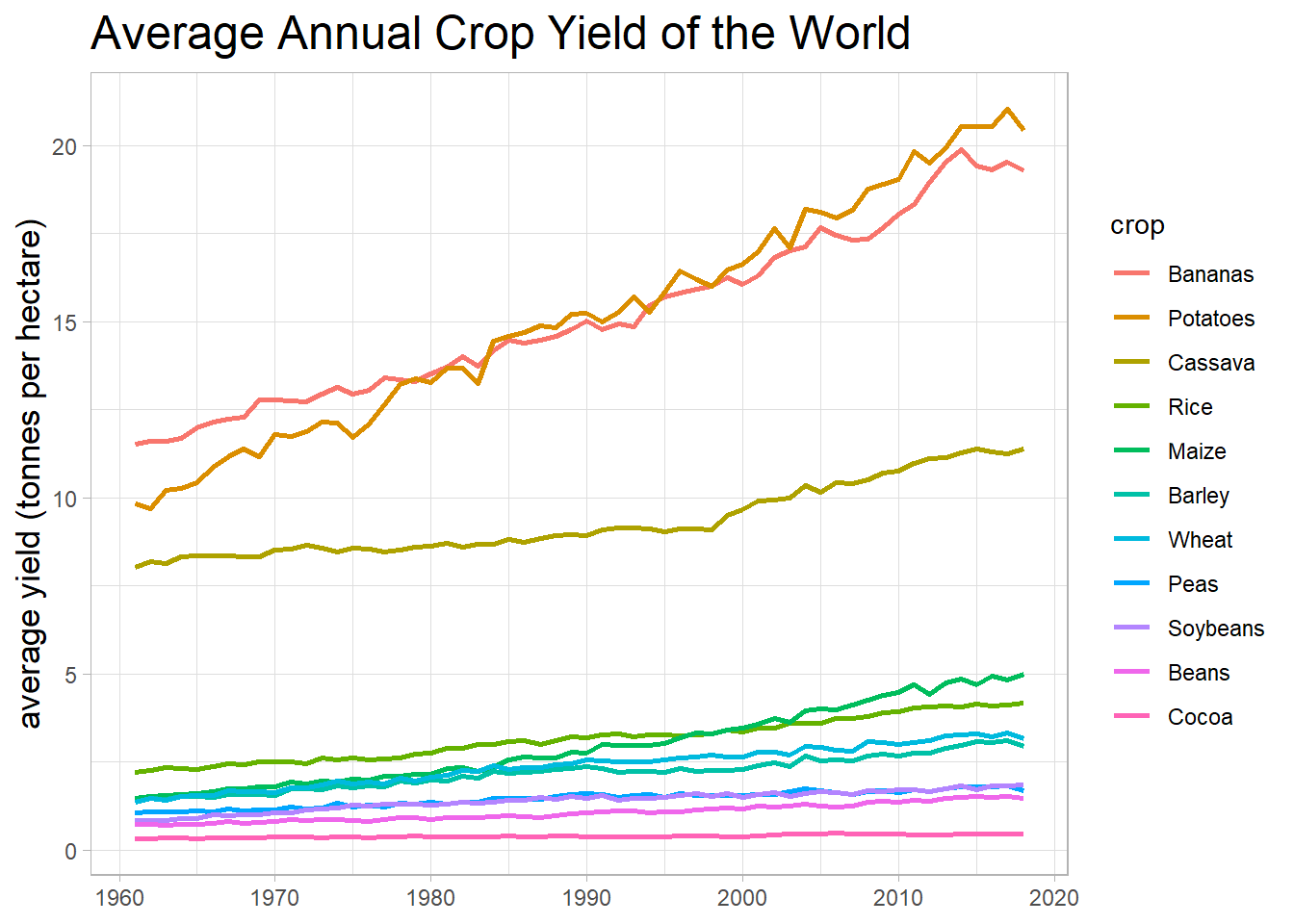
Average crop yield from 1960 - 2020 continentwide
countrycode::codelist %>%
  select(continent, cow.name, cowc) %>%
  right_join(country_crop, by = c(cowc = "code")) %>%
  distinct() %>%
  group_by(continent, crop, year) %>%
  summarize(yield = mean(yield, na.rm = T)) %>%
  ungroup() %>%
  mutate(crop = fct_reorder(crop, -yield, max)) %>%
  ggplot(aes(year, yield, color = crop)) +
  geom_line(size = 1) +
  facet_wrap(~continent) +
  theme(plot.title = element_text(size = 18),
        strip.text = element_text(size = 15),
        axis.title = element_text(size = 13)) +
  labs(x = NULL,
       y = "average yield (tonnes per hectare)",
       title = "Average Annual Crop Yield of All Continents")
The following crop_yields_50_years is inspired by David Robinson’s code.
crop_yields_50_years <- country_crop %>%
  arrange(entity, year) %>%
  filter(year >= 1968) %>%
  group_by(entity, code, crop) %>%
  summarize(first_year = min(year),
            last_year = max(year),
            yield_start = first(yield),
            yield_end = last(yield)) %>%
  filter(!is.na(code),
         first_year == 1968) %>%
  ungroup() %>%
  mutate(yield_ratio = yield_end/yield_start)
crop_yields_50_years %>%
ggplot(aes(yield_start, yield_end, color = crop)) +
geom_point() +
geom_text(aes(label = entity), check_overlap = T, hjust = 1, vjust = 1, size = 3) +
geom_abline(color = "red") +
facet_wrap(~crop) +
scale_x_log10() +
scale_y_log10() +
labs(x = "yield in 1968",
y = "yield in 2018",
title = "How had the Crop Yield been Changed in 50 Years?",
subtitle = "All yields are compared to the respective yield in 1961") +
theme(legend.position = "none",
strip.text = element_text(size = 15),
plot.title = element_text(size = 18))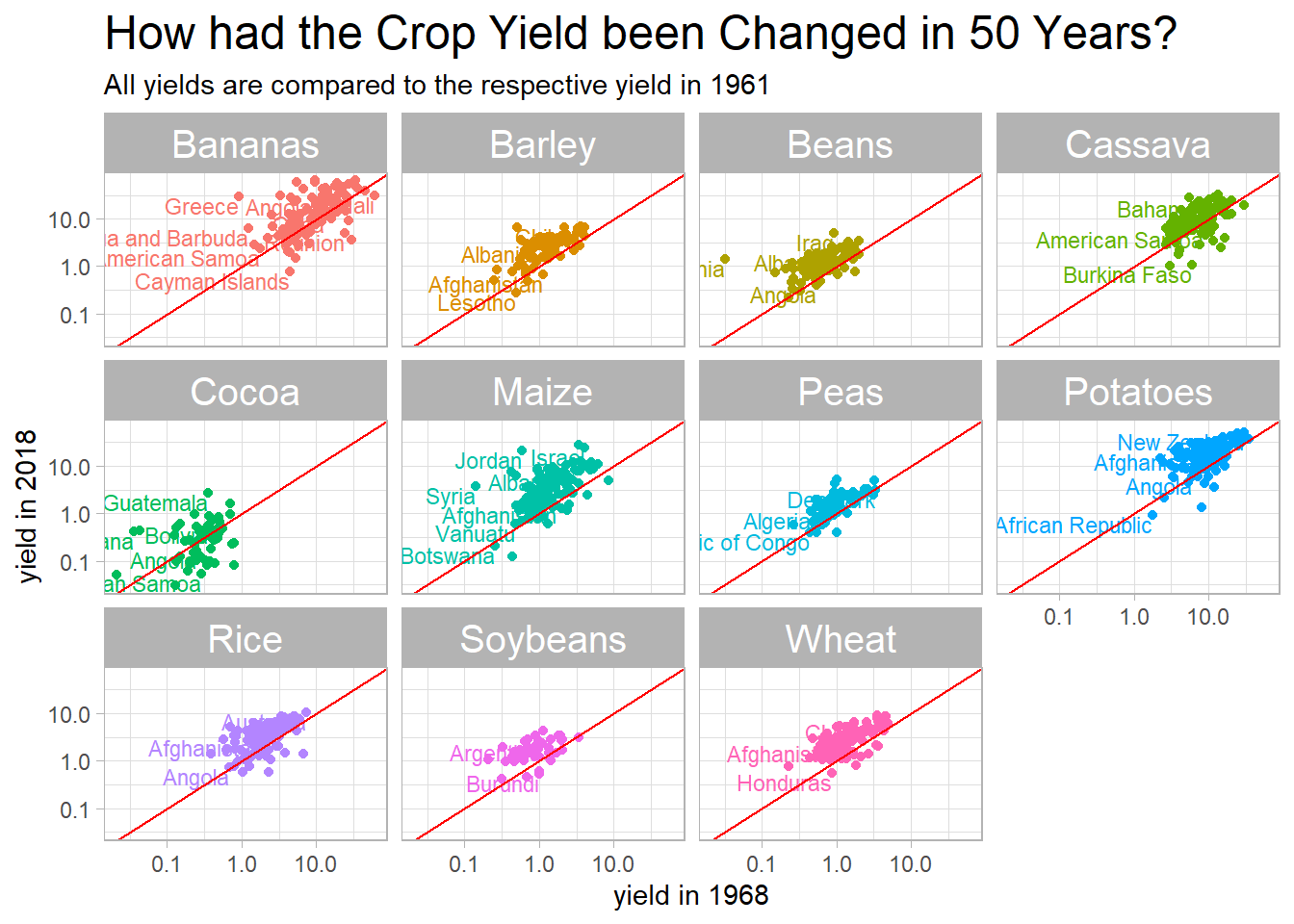
Yield ratio:
crop_yields_50_years %>%
  mutate(crop = fct_reorder(crop, yield_ratio, median, na.rm = T)) %>%
  ggplot(aes(yield_ratio, crop)) +
  geom_boxplot() +
  scale_x_log10() +
  labs(x = "yield ratio between 2018 and 1968",
       y = NULL,
       title = "Crop Ratio within 50 Years")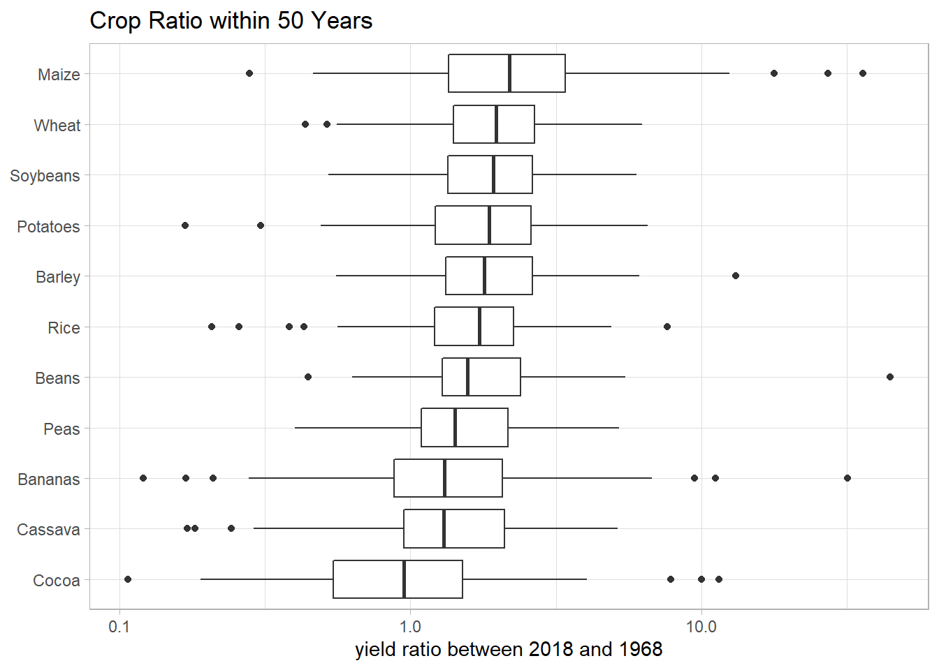
Working on arable_land:
arable_land %>%
  rename(arable_land = 4) %>%
  filter(Entity %in% c("Africa", "Americas", "Asia", "Europe", "Oceania")) %>%
  janitor::clean_names() %>%
  mutate(entity = fct_reorder(entity, -arable_land, max)) %>%
  ggplot(aes(year, arable_land, color = entity)) +
  geom_line(size = 1) +
  labs(y = "arable land percentage",
       color = "",
       title = "Arable Land Percentage Compared to 1960") +
  scale_y_continuous(label = scales::percent)
What is shocking about the above plot is Asia’s arable land has dropped dramatically since 1960, although all continents have seen the similar trend. It is reasonable to assume that some techonology had helped agriculture significantly.
Working on land_use:
land_use %>%
  select(1:3, 6) %>%
  rename(total_pop = 4) %>%
  inner_join(countrycode::codelist %>% select(continent, cow.name, cowc), by = c(Code = "cowc", Entity = "cow.name")) %>%
  distinct() %>%
  filter(str_detect(Year, "\\d\\d\\d\\d")) %>%
  group_by(Year, continent) %>%
  summarize(yearly_total_pop = sum(total_pop, na.rm = T)) %>%
  ungroup() %>%
  mutate(Year = as.numeric(Year)) %>%
  filter(Year > 1960,
         !is.na(continent)) %>%
  mutate(continent = fct_reorder(continent, -yearly_total_pop, sum)) %>%
  ggplot(aes(Year, yearly_total_pop, color = continent)) +
  geom_line(size = 1) +
  scale_y_log10() +
  labs(x = NULL,
       y = "total population",
       title = "Annual Total Population across Five Major Continents") +
  theme(plot.title = element_text(size = 18),
        strip.text = element_text(size = 15),
        axis.title = element_text(size = 13))
All continents expreienced population growth except Europe during 1960-2020.
land_use %>%
  rename(land_for_cereal = 5) %>%
  mutate(Year = as.numeric(Year)) %>%
  filter(Year > 1960) %>%
  filter(Code %in% c("USA", "CHN", "GBR", "JPN", "THA")) %>%
  mutate(Code = fct_reorder(Code, -land_for_cereal, sum, na.rm = T)) %>%
  ggplot(aes(Year, land_for_cereal, color = Code)) +
  geom_line(size = 1) +
  labs(x = NULL,
       y = "land for cereal",
       title = "The Relative Land for Cereal within Country Compared to 1960")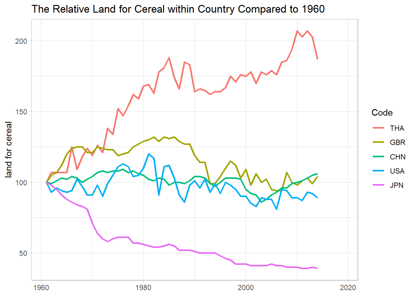
Thailand’s land for cereal had been more than doubled near 2010, yet its Japanese counterpart was decreased dramatically.
Working on fertilizer:
fertilizer %>%
  rename(cereal_yield = 4,
         fertilizer_use_kg = 5) %>%
  ggplot(aes(fertilizer_use_kg, cereal_yield, color = Year)) +
  geom_point() +
  scale_x_log10(label = scales::number) +
  scale_y_log10() +
  geom_smooth(method = "lm", se = F) +
  scale_color_gradient(low = "green",
                       high = "red") +
  labs(x = "fertilizer use (kg/hectare)",
       y = "cereal yield (ton/hectare)")
It seems like more fertilizer used, more cereal yielded. Also, as time progressed, fertilizer was used more and more.