The Show of Friends Data Visualization
This blog post is an interesting one. It analyzes the show Friends from TidyTuesday.
library(tidyverse)
library(patchwork)
library(tidytext)
library(widyr)
library(tidylo)
theme_set(theme_light())
friends <- read_csv('https://raw.githubusercontent.com/rfordatascience/tidytuesday/master/data/2020/2020-09-08/friends.csv')
friends_emotions <- read_csv('https://raw.githubusercontent.com/rfordatascience/tidytuesday/master/data/2020/2020-09-08/friends_emotions.csv')
friends_info <- read_csv('https://raw.githubusercontent.com/rfordatascience/tidytuesday/master/data/2020/2020-09-08/friends_info.csv') %>%
mutate(title = str_trim(str_remove_all(str_to_title(title), "The One With|The One Where")))Working on friends_into:
How popular is each episode?
- The 1st way to show:
friends_info %>%
  pivot_longer(c(7,8), names_to = "metric") %>%
  mutate(metric = str_replace_all(metric, "_", " ")) %>%
  ggplot(aes(air_date, value, color = metric)) +
  geom_line() +
  geom_text(aes(label = title),
            check_overlap = T, size = 3, alpha = 0.5,
            hjust = 1, vjust = 1) +
  geom_point() +
  facet_wrap(~metric, scales = "free_y") +
  labs(x = "air date",
       y = NULL,
       title = "How Popular was each Friends Episode?") +
  theme(legend.position = "none",
        strip.text = element_text(size = 15),
        plot.title = element_text(size = 18))
- The 2nd way to show:
friends_info %>%
  ggplot(aes(air_date, imdb_rating)) +
  geom_line() +
  geom_point(aes(size = us_views_millions, color = factor(season))) +
  geom_text(aes(label = title),
            check_overlap = T, size = 3, alpha = 0.5,
            hjust = 1, vjust = 1) +
  scale_color_discrete(guide = "none") +
  theme(plot.title = element_text(size = 18)) +
  labs(size = "US views (millions)",
       x = "air date",
       y = "IMDB rating",
title = "How Popular was each Friends Episode?") 
Episode Director:
directed_boxplot <- function(column) {
  friends_info %>%
  add_count(directed_by) %>%
  filter(n > 5) %>%
  mutate(directed_by = fct_reorder(directed_by, {{ column }}, median, na.rm = T)) %>%
  ggplot(aes({{ column }}, directed_by)) +
  geom_boxplot()
}

directed_boxplot(imdb_rating) / directed_boxplot(us_views_millions)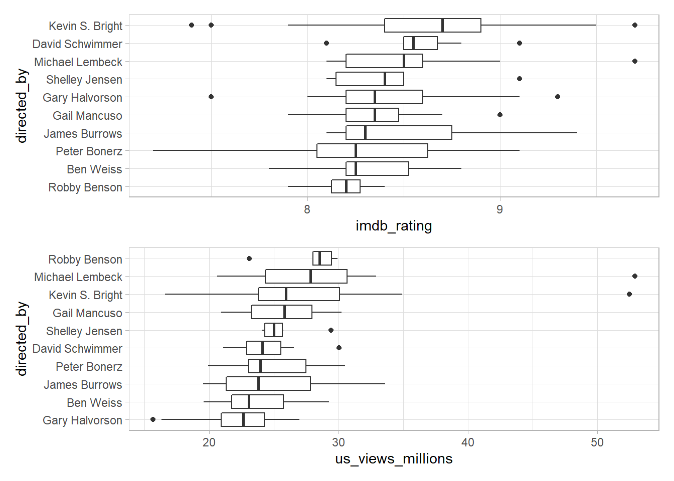
There is another way to generate the faceted plot above:
plots <- map(syms(list("us_views_millions", "imdb_rating")), directed_boxplot)
reduce(plots, `/`)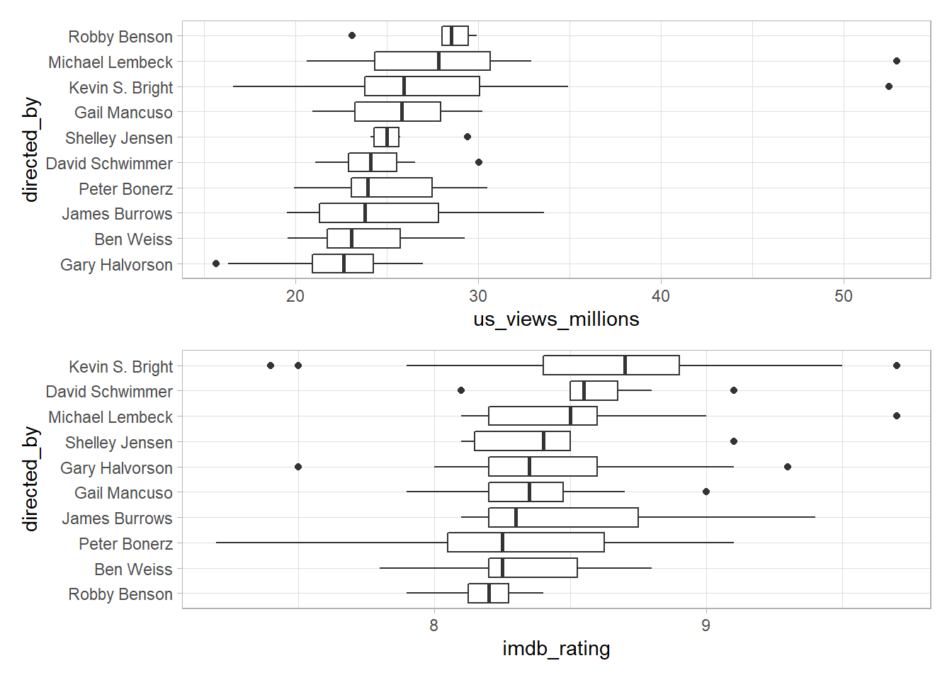
friends_info %>%
  filter(fct_lump(directed_by, n = 9) != "Other") %>%
  mutate(directed_by = fct_reorder(directed_by, -us_views_millions, sum)) %>%
  ggplot(aes(us_views_millions, imdb_rating, color = factor(season))) +
  geom_point() +
  geom_text(aes(label = title), vjust = 1, hjust = 0.8,
            check_overlap = T, size = 3.5) +
  facet_wrap(~directed_by, ncol = 5) +
  labs(x = "US views (millions)",
       y = "IMDB rating",
       color = "season",
       title = "Top 10 Directors") +
  theme(strip.text = element_text(size = 13),
        plot.title = element_text(size = 18))
Writers’ information:
friends_info %>%
  mutate(written_by = str_remove_all(written_by, "Story by.+$|Teleplay by.+$")) %>%
  separate_rows(written_by, sep = " & ") %>%
  add_count(written_by) %>%
  filter(written_by != "",
         n > 5) %>%
  pivot_longer(cols = c(7:8)) %>%
  mutate(name = str_to_upper(str_replace_all(name, "_", " ")),
         written_by = reorder_within(written_by, value, name)) %>%
  ggplot(aes(value, written_by)) +
  geom_boxplot() +
  scale_y_reordered() +
  facet_wrap(~name, scales = "free") +
  labs(x = NULL,
       y = "episode writer",
       title = "Episode Writers' Performance") +
  theme(strip.text = element_text(size = 13),
        plot.title = element_text(size = 18))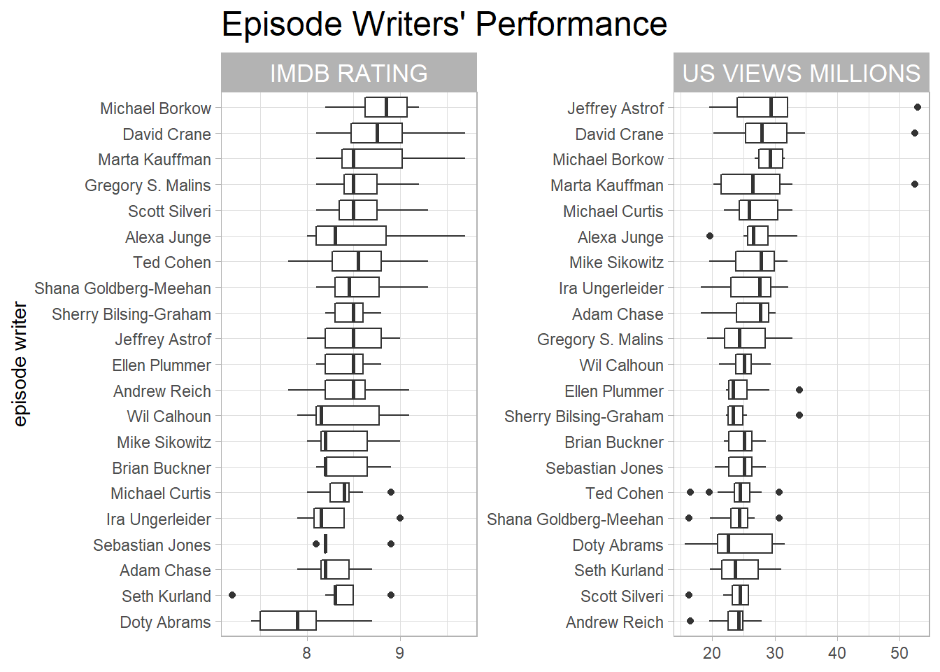
Combining friends and friends_emotions:
friends_joined <- friends %>%
  left_join(friends_emotions, by = c("season", "episode", "scene", "utterance")) %>%
  left_join(friends_info %>% select(season, episode, imdb_rating), by = c("season", "episode")) %>%
  filter(fct_lump(speaker, n = 6) != "Other")

friends_joined
## # A tibble: 51,047 x 8
## text speaker season episode scene utterance emotion imdb_rating
## <chr> <chr> <dbl> <dbl> <dbl> <dbl> <chr> <dbl>
## 1 There's nothing t~ Monica~ 1 1 1 1 <NA> 8.3
## 2 C'mon, you're goi~ Joey T~ 1 1 1 2 <NA> 8.3
## 3 All right Joey, b~ Chandl~ 1 1 1 3 <NA> 8.3
## 4 Wait, does he eat~ Phoebe~ 1 1 1 4 <NA> 8.3
## 5 Just, 'cause, I d~ Phoebe~ 1 1 1 6 <NA> 8.3
## 6 Okay, everybody r~ Monica~ 1 1 1 7 <NA> 8.3
## 7 Sounds like a dat~ Chandl~ 1 1 1 8 <NA> 8.3
## 8 Alright, so I'm b~ Chandl~ 1 1 1 10 <NA> 8.3
## 9 Then I look down,~ Chandl~ 1 1 1 12 <NA> 8.3
## 10 Instead of...? Joey T~ 1 1 1 13 <NA> 8.3
## # ... with 51,037 more rowsWho speaks the most in each season?
friends_joined %>%
  mutate(season = fct_reorder(paste("Season", season), season)) %>%
  count(speaker, season, sort = T) %>%
  mutate(speaker = reorder_within(speaker, n, season)) %>%
  ggplot(aes(n, speaker)) +
  geom_col() +
  scale_y_reordered() +
  facet_wrap(~season, scales = "free_y") +
  labs(x = "# of lines",
       y = NULL,
       title = "Who Speaks the Most?") +
  theme(strip.text = element_text(size = 15),
        plot.title = element_text(size = 18))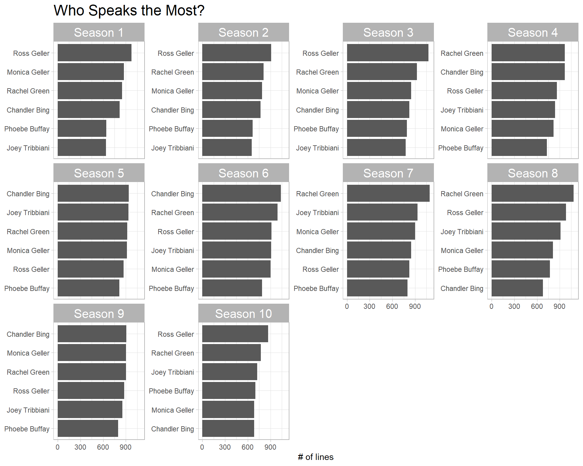
It’s either Ross or Chandler or Rachel who speaks the most!
friends_joined %>%
  group_by(season, episode, speaker) %>%
  summarize(episode_line_per_speaker = n(),
            imdb_rating) %>%
  ungroup() %>%
  distinct() %>%
  mutate(episode = paste0("E", episode, "(",imdb_rating, ")"),
         season = paste("Season", season)) %>%
  mutate(season = fct_reorder(season, parse_number(season)),
         episode = fct_reorder(episode, parse_number(episode))) %>%
  ggplot(aes(episode_line_per_speaker, episode, fill = speaker)) +
  geom_col() +
  facet_wrap(~season, scales = "free_y") +
  labs(x = "episode line",
       y = NULL,
       fill = NULL,
       title = "The Overall Distribution of Lines Across All Friends Episodes",
       subtitle = "The numbers in the bracket refer to IMDB rating") +
  theme(plot.title = element_text(size = 18),
strip.text = element_text(size = 15)) 
TF-IDF
friends_joined %>%
  unnest_tokens(word, text) %>%
  anti_join(stop_words) %>%
  filter(!str_detect(word, "\\d")) %>%
  count(speaker, word, sort = T) %>%
  bind_tf_idf(word, speaker, n) %>%
  group_by(speaker) %>%
  slice_max(tf_idf, n = 20, with_ties = F) %>%
  ungroup() %>%
  mutate(word = reorder_within(word, tf_idf, speaker),
         speaker = fct_reorder(speaker, -tf_idf, sum)) %>%
  ggplot(aes(tf_idf, word, fill = speaker)) +
  geom_col(show.legend = F) +
  scale_y_reordered() +
  facet_wrap(~speaker, scales = "free_y") +
  theme(strip.text = element_text(size = 15),
        plot.title = element_text(size = 18)) +
  labs(x = "TF-IDF",
       y = NULL,
       title = "Top 20 Words with the Largest TF-IDF Values for 6 Major Characters")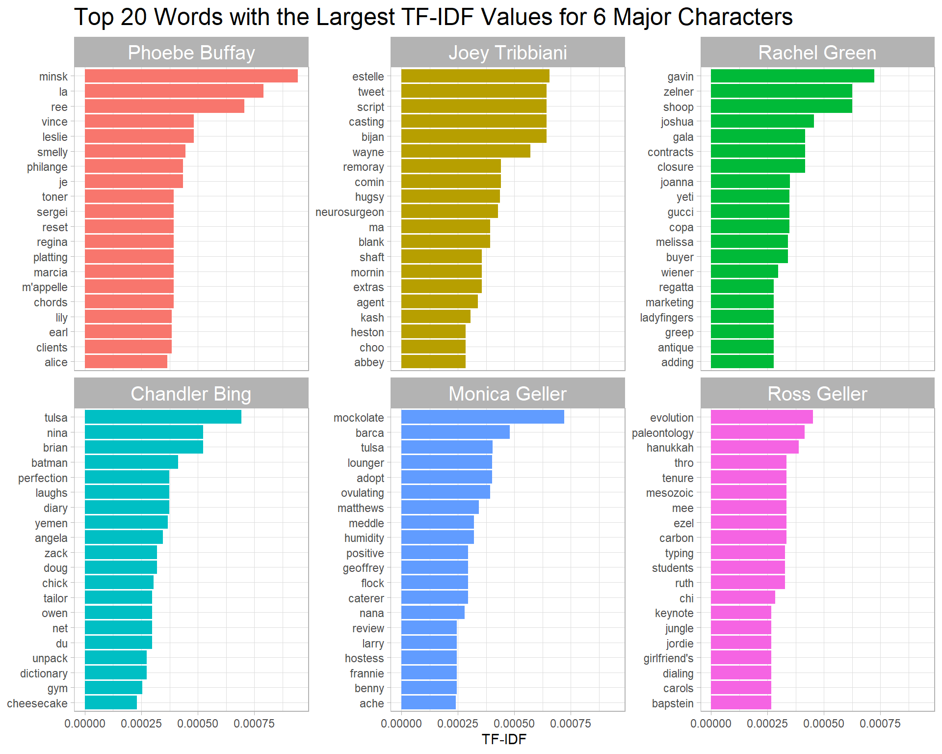
Weighted log odds
After being inspired by David Robinson’s code and Julia Silge’s tidylo package, I have:
friends_joined %>%
  unnest_tokens(word, text) %>%
  anti_join(stop_words) %>%
  filter(!str_detect(word, "\\d")) %>%
  count(speaker, word, sort = T) %>%
  bind_log_odds(speaker, word, n) %>%
  filter(n > 20) %>%
  group_by(speaker) %>%
  slice_max(log_odds_weighted, n = 15) %>%
  mutate(word = reorder_within(word, log_odds_weighted, speaker)) %>%
  ggplot(aes(log_odds_weighted, word, fill = speaker)) +
  geom_col(show.legend = F) +
  scale_y_reordered() +
  facet_wrap(~speaker, scales = "free_y") +
  labs(x = "weighted log odds",
       y = NULL,
       title = "Weighted Log Odds for 6 Main Characters") +
  theme(strip.text = element_text(size = 15),
        plot.title = element_text(size = 18))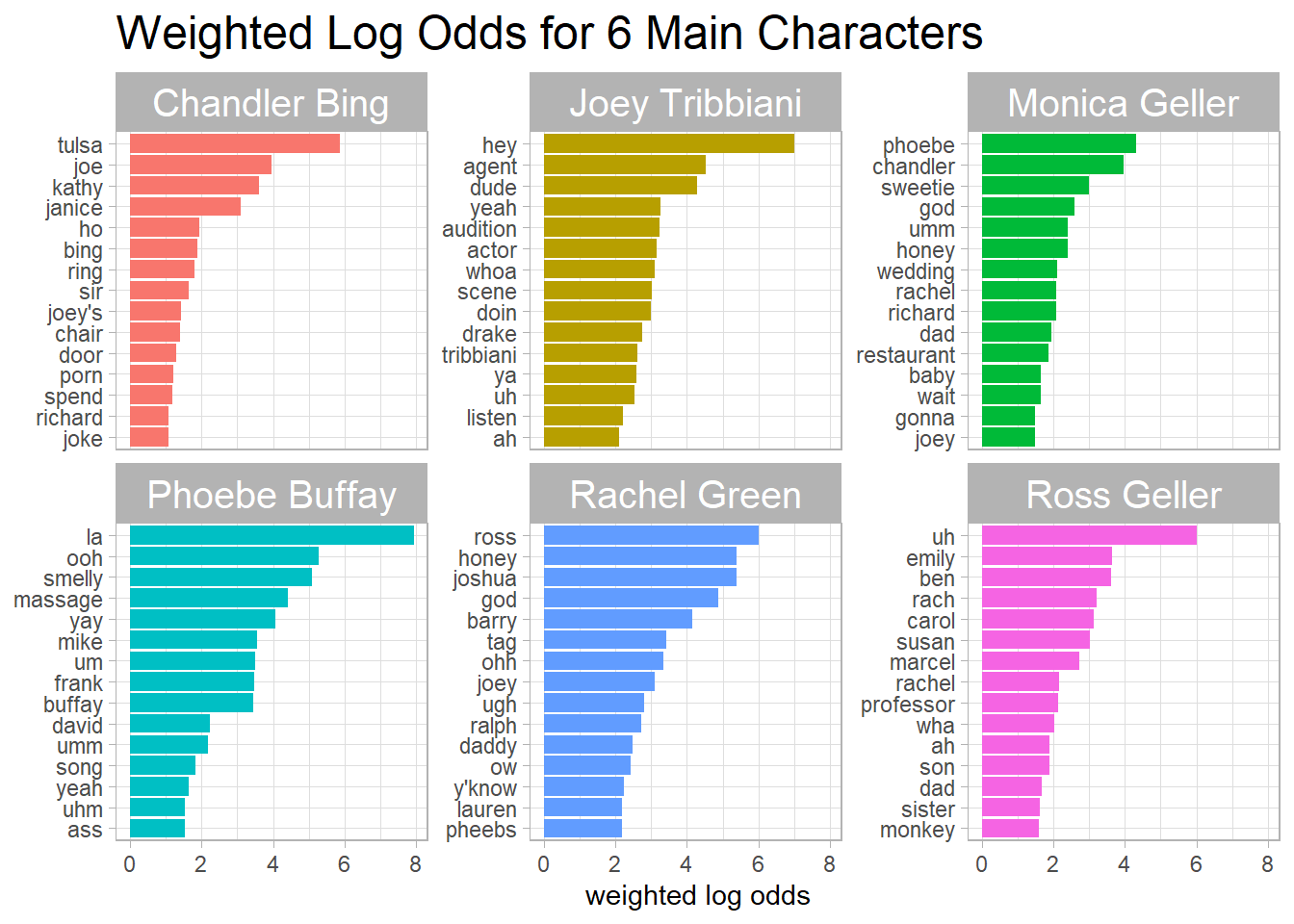
It seems like log_odds_weighted is analogous to TF-IDF, and it is just another way to show which words are more “targeted” from a specific speaker.
The following code is inspired by David Robinson’s cdoe to see which characters tend to appear together by using pairwise_cor() from the widyr package.
friends %>%
  filter(fct_lump(speaker, n = 6) != "Other") %>%
  unite(scene_id, season, episode, scene) %>%
  count(speaker, scene_id, sort =T) %>%
  pairwise_cor(speaker, scene_id, n) %>%
  mutate(item1 = reorder_within(item1, correlation, item2)) %>%
  ggplot(aes(correlation, item1, fill = item2)) +
  geom_col(show.legend = F) +
  scale_y_reordered() +
  facet_wrap(~item2, scales = "free_y") +
  labs(y = NULL,
       title = "Who Tends to be Appearing Together?") +
  theme(strip.text = element_text(size = 15),
        plot.title = element_text(size = 18))
Rachel and Chandler appear together least in the show.