US Spending on Kids Data Visualization
This blog post analyzes how much money each state in the U.S. spent on kids through various programs between 1997 and 2016 (20-year period). As usual, the data comes from TidyTuesday.
library(tidyverse)
library(geofacet)
library(scales)
library(tidytext)
theme_set(theme_light())
kids <- read_csv('https://raw.githubusercontent.com/rfordatascience/tidytuesday/master/data/2020/2020-09-15/kids.csv') %>%
filter(inf_adj > 0) %>%
mutate(variable = str_to_title(str_replace(variable, "_", " "))) %>%
left_join(tibble(state = state.name, state_abb = state.abb), by = "state") %>%
mutate(state_abb = if_else(is.na(state_abb), "DC", state_abb),
across(raw:inf_adj_perchild, ~ . * 1000))Overview of the state governments’ spending on kids:
kids %>%
  filter(!is.na(inf_adj),
         fct_lump(variable, n = 6, w = inf_adj)!= "Other") %>%
  mutate(variable = fct_reorder(variable, -inf_adj, sum)) %>%
  ggplot(aes(year, inf_adj, color = variable)) +
  geom_line(size = 1) +
  scale_y_continuous(labels = dollar) +
  facet_geo(~state_abb, scales = "free_y") +
  theme(axis.text.x = element_text(angle = 90),
        strip.text = element_text(size = 15, face = "bold"),
        plot.title = element_text(size = 18)) +
  labs(y = "adjusted spending",
       color = NULL,
       title = "State-wise Government Spending on 6 Major Categories on Kids (1997 - 2016)")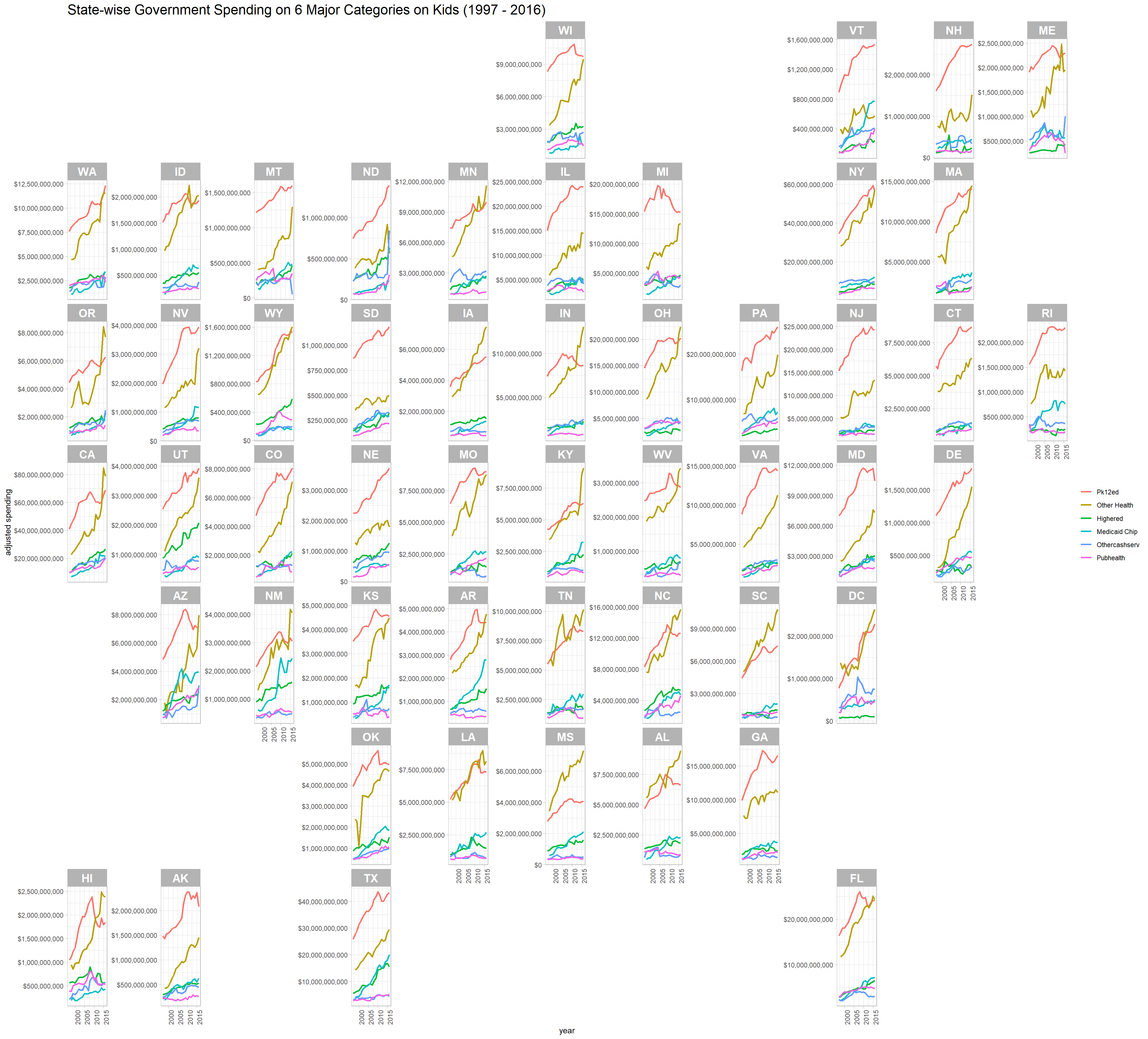
The spending on some categories (e.g,Pk12ed) have risen up significantly across all states, yet others remain relatively the same level throughout the years.
kids %>%
  filter(fct_lump(variable, n = 6, w = inf_adj_perchild) != "Other") %>%
  mutate(variable = fct_reorder(variable, -inf_adj_perchild, sum)) %>%
  ggplot(aes(year, inf_adj_perchild, color = variable)) +
  geom_line(size = 0.7) +
  scale_y_continuous(labels = dollar) +
  facet_geo(~state_abb) +
  theme(axis.text.x = element_text(angle = 90),
        strip.text = element_text(size = 15, face = "bold"),
        plot.title = element_text(size = 18)) +
  labs(y = "adjusted spending per child",
       color = NULL,
       title = "State-wise Government Spending on 6 Major Categories on Kids (1997 - 2016)")
Although total spending has been rising, the adjusted invenstement on children per captia remains stable. One possible reason is there were more children in the later time interval than the earlier.
Comparing 1997 and 2016 spending:
kids %>%
  filter(year %in% c(1997, 2016)) %>%
  select(1, 2,3,5,7) %>%
  pivot_wider(names_from = "year",
              values_from = "inf_adj") %>%
  mutate(ratio = (`2016` - `1997`)/`1997`) %>%
  group_by(state, state_abb) %>%
  slice_max(ratio, n = 5) %>%
  ungroup() %>%
  mutate(variable = reorder_within(variable, ratio, state_abb)) %>%
  ggplot(aes(ratio, variable, fill = variable)) +
  geom_col(show.legend = F) +
  scale_y_reordered() +
  scale_x_continuous(labels = percent) +
  facet_geo(~state_abb, scales = "free") +
  labs(x = "2016 to 1997 ratio",
       y = "spending sector",
       title = "State-wise Top 5 Largest Increase Among the 20 Year Period") +
  theme(axis.text.x = element_text(angle = 90),
        plot.title = element_text(size = 18),
        strip.text = element_text(size = 15))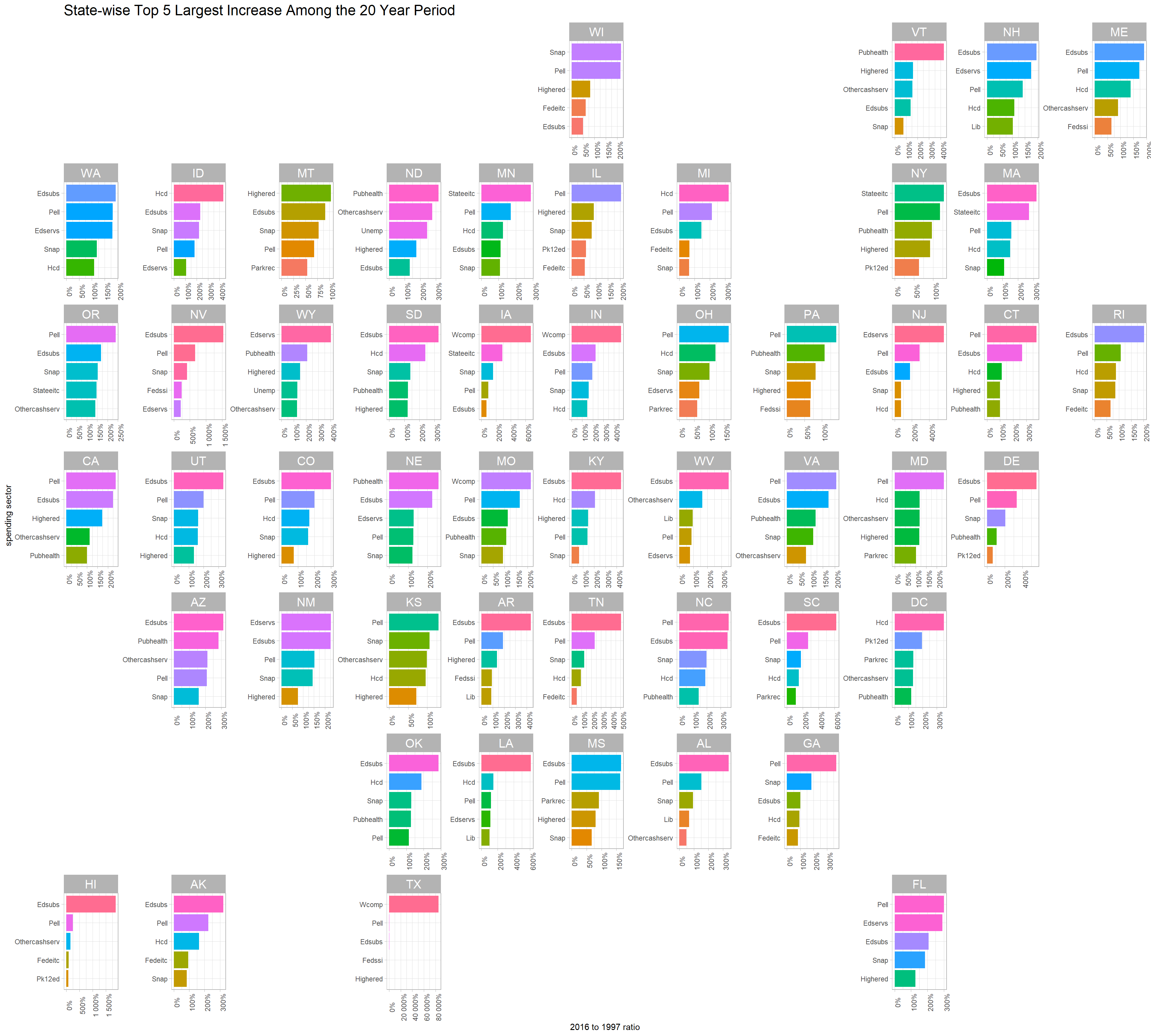
Here we get the number of kids each year in each state:
kids_count <- kids %>%
  mutate(num_of_kids = ceiling(inf_adj/inf_adj_perchild)) %>%
  distinct(year, state_abb, .keep_all = T) %>%
  select(state_abb, year, num_of_kids)

kids_count
## # A tibble: 1,020 x 3
## state_abb year num_of_kids
## <chr> <dbl> <dbl>
## 1 AL 1997 1187268
## 2 AK 1997 196883
## 3 AZ 1997 1303319
## 4 AR 1997 718408
## 5 CA 1997 9558726
## 6 CO 1997 1084928
## 7 CT 1997 854740
## 8 DE 1997 196901
## 9 DC 1997 127063
## 10 FL 1997 3681284
## # ... with 1,010 more rowsTotal number of kids across the U.S.:
kids_count %>%
  group_by(year) %>%
  summarize(num_of_kids_year = sum(num_of_kids)) %>%
  ggplot(aes(year, num_of_kids_year)) +
  geom_line() +
  geom_point() +
  scale_y_continuous(labels = comma) +
  labs(y = "# of kids",
       title = "Yearly # of Kids in the U.S.")
Total number of kids across all states:
kids_count %>%
  ggplot(aes(year, num_of_kids, color = state_abb)) +
  geom_line() +
  geom_point() +
  facet_geo(~state_abb, scales = "free_y") +
  theme(axis.text.x = element_text(angle = 90),
        legend.position = "none",
        plot.title = element_text(size = 18),
        strip.text = element_text(size = 15)) +
  labs(y = "# of kids",
title = "State-wise # of Kids") 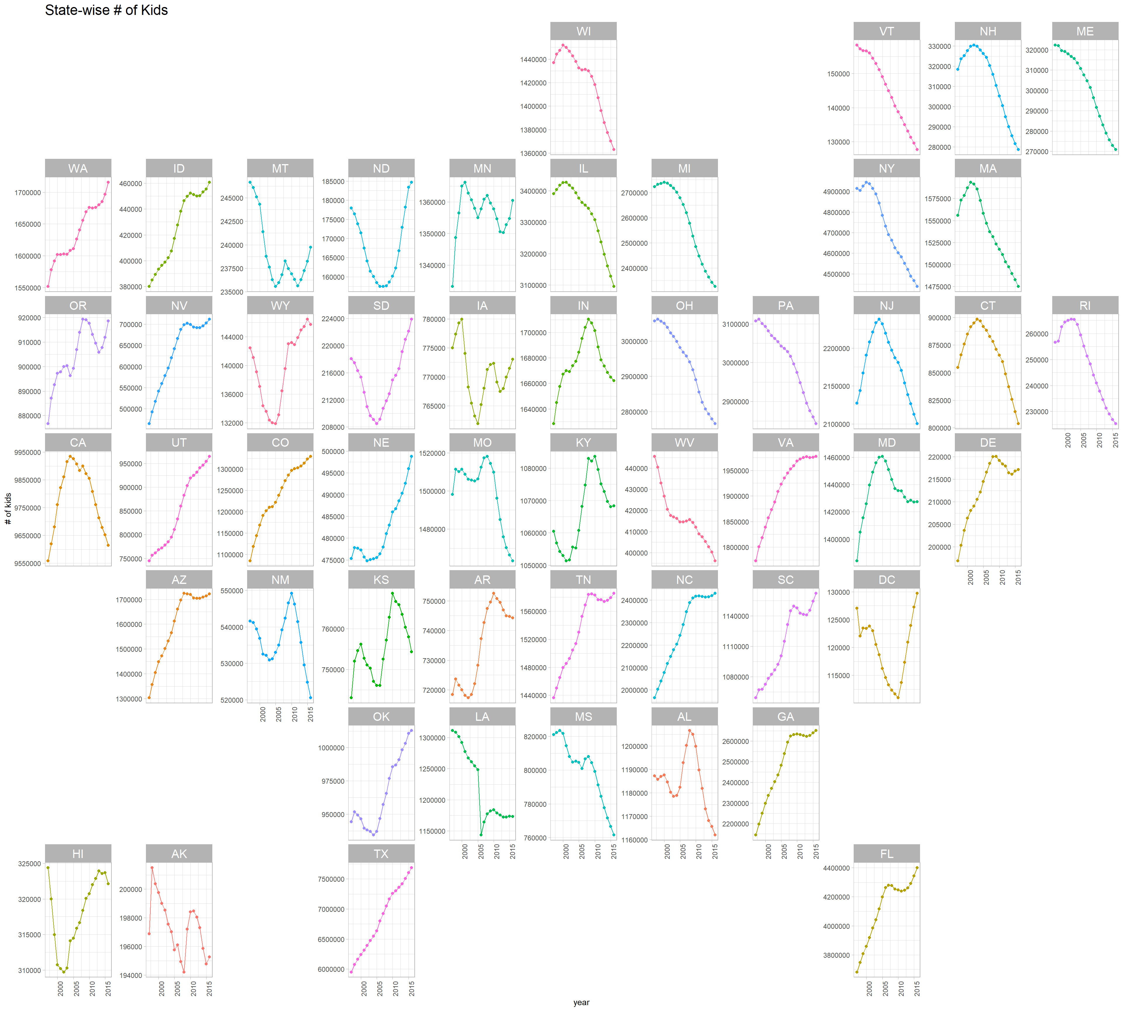
Kids’ growth rate:
kids_count %>%
  group_by(state_abb) %>%
  mutate(previous_num_of_kids = lag(num_of_kids),
         growth_rate = (num_of_kids - previous_num_of_kids)/previous_num_of_kids) %>%
  filter(!is.na(growth_rate)) %>%
  ungroup() %>%
  ggplot(aes(year, growth_rate, color = state_abb)) +
  geom_line(size = 1) +
  scale_y_continuous(labels = percent) +
  facet_geo(~state_abb) +
  theme(axis.text.x = element_text(angle = 90),
        legend.position = "none",
        plot.title = element_text(size = 18),
        strip.text = element_text(size = 15)) +
  labs(y = "rate of kids' growth",
       title = "State-wise Yearly Growth Rate for Kids",
subtitle = "Growth rate compares the current year to the previous year") 
All states remain relatively stable on kids’ growth rate. What is worth noting is that the state of LA had a sudden drop on kids’ growth rate. I guess the reason was the Katrina Hurricane.
Let’s look at Ohio in particular:
ohio <- kids %>%
  filter(state == "Ohio")

ohio
## # A tibble: 428 x 7
## state variable year raw inf_adj inf_adj_perchild state_abb
## <chr> <chr> <dbl> <dbl> <dbl> <dbl> <chr>
## 1 Ohio Pk12ed 1997 10213866000 1.46e10 4764. OH
## 2 Ohio Highered 1997 1706351000 2.43e 9 796. OH
## 3 Ohio Edsubs 1997 553903000 7.90e 8 258. OH
## 4 Ohio Edservs 1997 219720000 3.13e 8 102. OH
## 5 Ohio Pell 1997 216774138 3.09e 8 101. OH
## 6 Ohio Headstartpriv 1997 134497015. 1.92e 8 62.7 OH
## 7 Ohio Tanfbasic 1997 697067991 9.94e 8 325. OH
## 8 Ohio Othercashserv 1997 2146527000 3.06e 9 1001. OH
## 9 Ohio Snap 1997 351871375 5.02e 8 164. OH
## 10 Ohio Socsec 1997 474286127. 6.76e 8 221. OH
## # ... with 418 more rowsohio %>%
mutate(variable = fct_reorder(variable, inf_adj, sum)) %>%
ggplot(aes(year, variable, fill = inf_adj)) +
geom_tile() +
scale_fill_gradient(low = "red",
high = "green",
trans = "log10",
labels = dollar) +
theme(panel.grid = element_blank()) +
labs(y = "spending sector",
fill = "adjusted spending",
title = "Ohio's Spendings on Kids")