Visualization on Himalayan Climbing Expeditions
Tue, Feb 15, 2022
4-minute read
This blog post anlayzes Himalayan Climbing data coming from TidyTuesday.
library(tidyverse)
library(tidytext)
library(widyr)
library(ggraph)
theme_set(theme_light())
members <- read_csv('https://raw.githubusercontent.com/rfordatascience/tidytuesday/master/data/2020/2020-09-22/members.csv')
expeditions <- read_csv('https://raw.githubusercontent.com/rfordatascience/tidytuesday/master/data/2020/2020-09-22/expeditions.csv') %>%
mutate(termination_reason = str_to_title(str_remove_all(termination_reason, "\\s\\(.*\\)|or\\s"))) %>%
separate_rows(termination_reason, sep = ", ") %>%
mutate(success_or_not = if_else(termination_reason == "Success", "success", "not success"))
peaks <- read_csv('https://raw.githubusercontent.com/rfordatascience/tidytuesday/master/data/2020/2020-09-22/peaks.csv') %>%
separate_rows(first_ascent_country, sep = ",\\s")Working on members:
members %>%
  distinct(expedition_id, year) %>%
  count(year, name = "num_of_climbs") %>%
  left_join(
    members %>%
      group_by(expedition_id, year) %>%
      summarize(n = n()) %>%
      ungroup() %>%
      count(year, wt = n, name = "num_of_climbers"),
    by = "year") %>%
  ggplot(aes(year, num_of_climbs)) +
  geom_line() +
  geom_point(aes(size = num_of_climbers)) +
  scale_x_continuous(breaks = seq(1900, 2020, 10)) +
  scale_size_continuous(range = c(1, 6), breaks = c(100, 200, 500, 1000, 2000)) +
  labs(x = NULL,
       y = "# of climbs",
       size = "# of yearly climbers",
       title = "Yearly # of Climbs and # of Climbers in Total") +
  theme(plot.title = element_text(size = 18))
Both # of climbs and # of climbers have increased dramatically in recent years.
Seasons:
members %>%
  filter(season != "Unknown") %>%
  distinct(expedition_id, year, season) %>%
  count(year, season, sort = T) %>%
  mutate(season = fct_reorder(season, -n, sum)) %>%
  ggplot(aes(year, n, color = season)) +
  geom_line(size = 1) +
  labs(x = NULL,
       y = "# of expeditions",
       title = "Yearly # of Expeditions per Season") +
  theme(plot.title = element_text(size = 18))
Both fall and spring have attracted much more climbers than other two seasons.
members %>%
  filter(fct_lump(citizenship, n = 10) != "Other",
         !is.na(sex),
         !is.na(age)) %>%
  mutate(sex = fct_recode(sex,
                          "Female" = "F",
                          "Male" = "M")) %>%
  mutate(citizenship = reorder_within(citizenship, age, sex, median)) %>%
  ggplot(aes(age, citizenship, fill = citizenship)) +
  geom_boxplot(show.legend = F) +
  scale_y_reordered() +
  facet_wrap(~sex, scales = "free_y") +
  labs(title = "Age Distributions among All Climbers from Top 10 Countries",
       subtitle = "Top countries are defined by # of climbers") +
  theme(strip.text = element_text(size = 15),
        plot.title = element_text(size = 18))
members %>%
  filter(highpoint_metres > 0) %>%
  distinct(year, highpoint_metres) %>%
  group_by(year) %>%
  summarize(highpoint = max(highpoint_metres, na.rm = T)) %>%
  ggplot(aes(year, highpoint)) +
  geom_line() +
  geom_point() +
  expand_limits(y = 0) +
  labs(y = "highpoint (meters)",
title = "The Annual Highest Point Achieved") 
Graph on countries:
set.seed(2022)

members %>%
  count(citizenship, peak_name, sort = T) %>%
  filter(n > 1000) %>%
  pairwise_cor(citizenship, peak_name, n, sort = T) %>%
  ggraph(layout = "fr") +
  geom_edge_link(aes(width = correlation, color = correlation), alpha = 0.5) +
  geom_node_point() +
  geom_node_text(aes(label = name), hjust = 1, vjust = -1, check_overlap = T, size = 5) +
  theme_void() +
  guides(color = "none", edge_color = "none") +
  labs(edge_color = "correlation",
       title = "How are countries correlated?") +
  theme(plot.title = element_text(size = 18))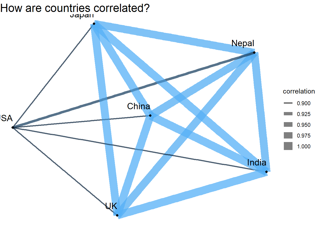
Death:
members %>%
  filter(died,
         fct_lump(expedition_role, n = 3)  != "Other") %>%
  count(death_cause, season, expedition_role, sort = T) %>%
  mutate(death_cause = reorder_within(death_cause, n, expedition_role)) %>%
  ggplot(aes(n, death_cause, fill = season)) +
  geom_col() +
  facet_wrap(~expedition_role, scales = "free_y") +
  scale_y_reordered() +
  labs(x = "# of deaths",
       y = "death cause",
       title = "The Reasons Why Climbers were Killed")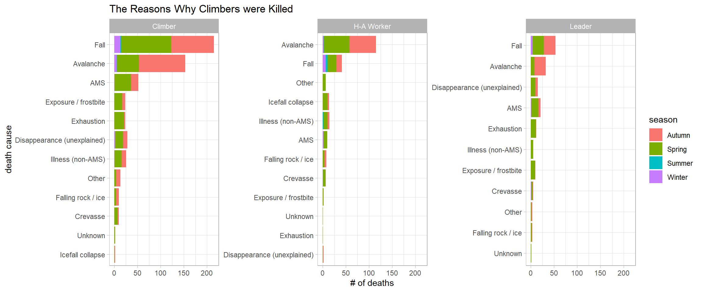
Working on expeditions:
What are the termination reasons?
expeditions %>%
  filter(fct_lump(termination_reason, n = 16) != "Other") %>%
  count(year, termination_reason, sort = T) %>%
  mutate(termination_reason = fct_reorder(termination_reason, -n, sum)) %>%
  ggplot(aes(year, n, color = termination_reason)) +
  geom_line() +
  geom_point() +
  facet_wrap(~termination_reason, ncol = 5) +
  theme(legend.position = "none") +
  labs(y = "# of expeditions terminated in this reason",
title = "How did Expeditions be Terminated?") 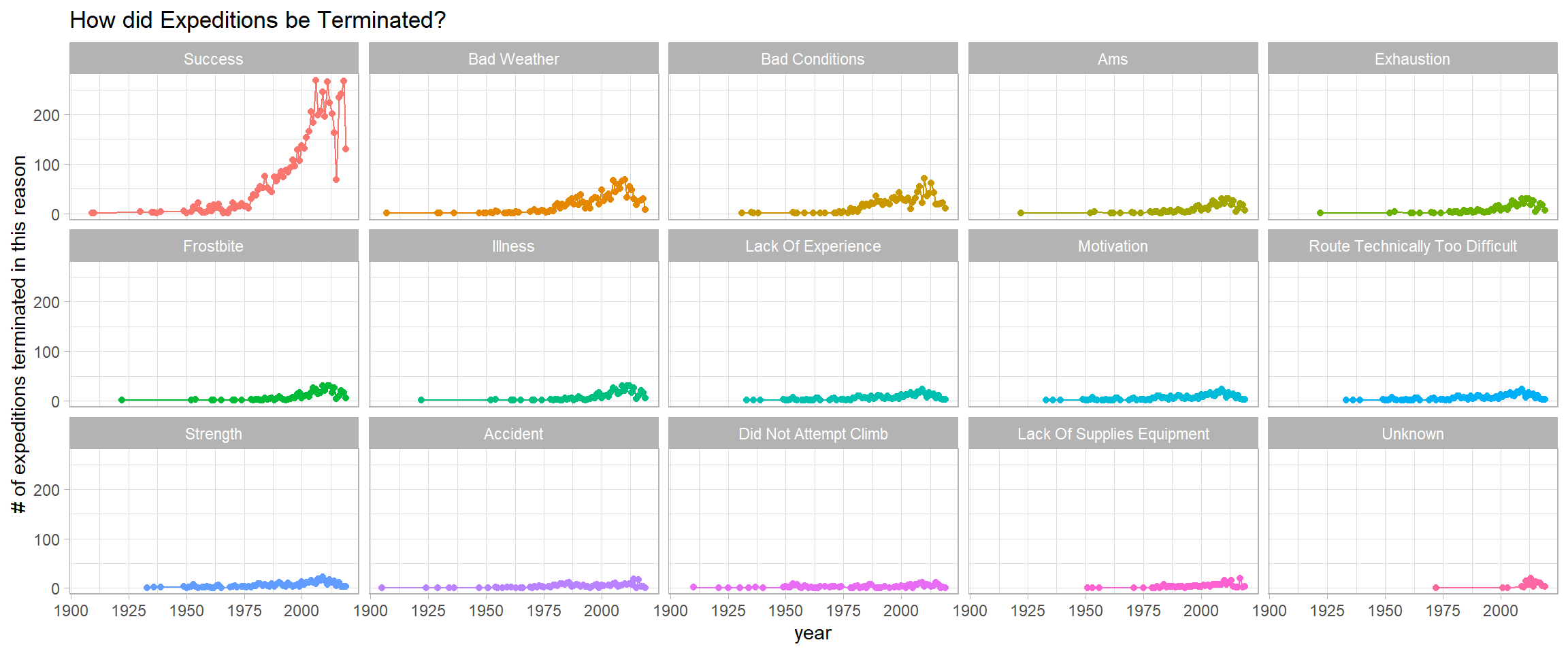
of members and success:
expeditions %>%
  ggplot(aes(members, success_or_not, fill = success_or_not)) +
  geom_boxplot(show.legend = F) +
  scale_x_log10() +
  labs(x = "# of members",
       y = "expediton result",
title = "More Team Members, Higher Chances for Success?") 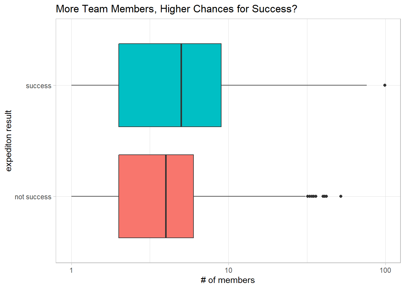
It looks like successful teams had more median members.
expeditions %>%
  filter(season %in% c("Autumn", "Spring")) %>%
  mutate(date = difftime(highpoint_date, basecamp_date, units = "days")) %>%
  ggplot(aes(date, fill = success_or_not)) +
  geom_histogram(alpha = 0.8) +
  facet_wrap(~season) +
  labs(x = "days",
       fill = NULL,
       title = "How Far Apart between Basecamp Date and Highpoint Date?")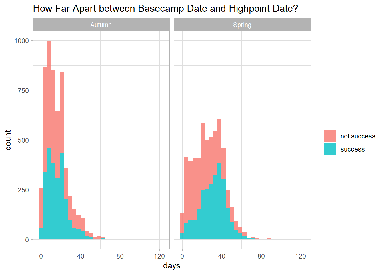
Working on peaks:
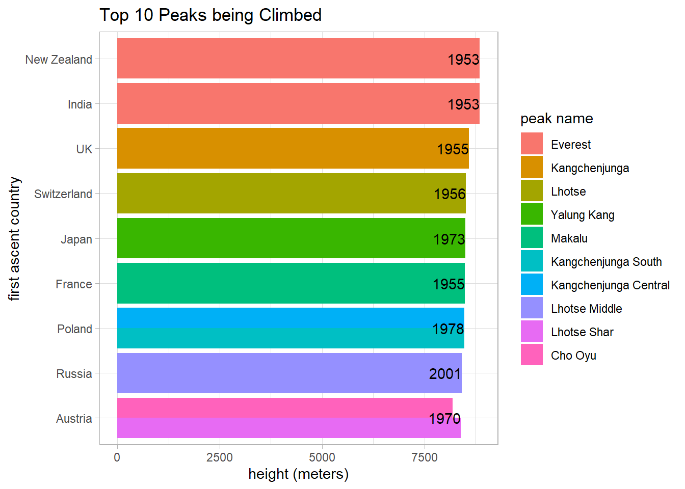
peaks %>%
  arrange(desc(height_metres),
          first_ascent_year) %>%
  head(11) %>%
  mutate(first_ascent_country = fct_reorder(first_ascent_country, height_metres),
         peak_name = fct_reorder(peak_name, -height_metres)) %>%
  ggplot(aes(first_ascent_country, height_metres, fill = peak_name)) +
  geom_col(position = "dodge") +
  geom_text(aes(label = first_ascent_year), hjust = 1, check_overlap = T) +
  coord_flip() +
  labs(y = "height (meters)",
       x = "first ascent country",
       fill = "peak name",
       title = "Top 10 Peaks being Climbed")