Analyzing Beyonce and Taylor Swift Lyrics
Sat, Feb 19, 2022
5-minute read
This blog post analyzes the lyrics from Beyonce and Taylor Swift, and the datasets are from TidyTuesday.
library(tidyverse)
library(lubridate)
library(scales)
library(tidytext)
library(tidylo)
theme_set(theme_light())
beyonce_lyrics <- read_csv('https://raw.githubusercontent.com/rfordatascience/tidytuesday/master/data/2020/2020-09-29/beyonce_lyrics.csv')
taylor_swift_lyrics <- read_csv('https://raw.githubusercontent.com/rfordatascience/tidytuesday/master/data/2020/2020-09-29/taylor_swift_lyrics.csv') %>%
rename(song = Title) %>%
janitor::clean_names()
sales <- read_csv('https://raw.githubusercontent.com/rfordatascience/tidytuesday/master/data/2020/2020-09-29/sales.csv')
charts <- read_csv('https://raw.githubusercontent.com/rfordatascience/tidytuesday/master/data/2020/2020-09-29/charts.csv') %>%
mutate(re_release = str_remove(re_release, "\\[.+\\]$"),
released = str_remove(released, "\\(.+$")) %>%
mutate(released = mdy(released),
re_release = mdy(re_release),
chart_position = as.numeric(chart_position)) %>%
rename(country_chart = chart,
album = title)Chart positions per country:
charts %>%
  ggplot(aes(released, chart_position, color = album)) +
  geom_line(aes(group = artist), size = 1) +
  geom_point() +
  geom_text(aes(label = album), hjust = 0, vjust = 1, check_overlap = T) +
  facet_grid(country_chart ~ artist) +
  scale_y_reverse() +
  scale_x_date(date_breaks = "2 years", date_labels = "%Y") +
  theme(legend.position = "none",
        strip.text = element_text(size = 15),
        plot.title = element_text(size = 18)) +
  labs(x = "released year",
       y = "chart position",
title = "Country-wise Album Chart Position") 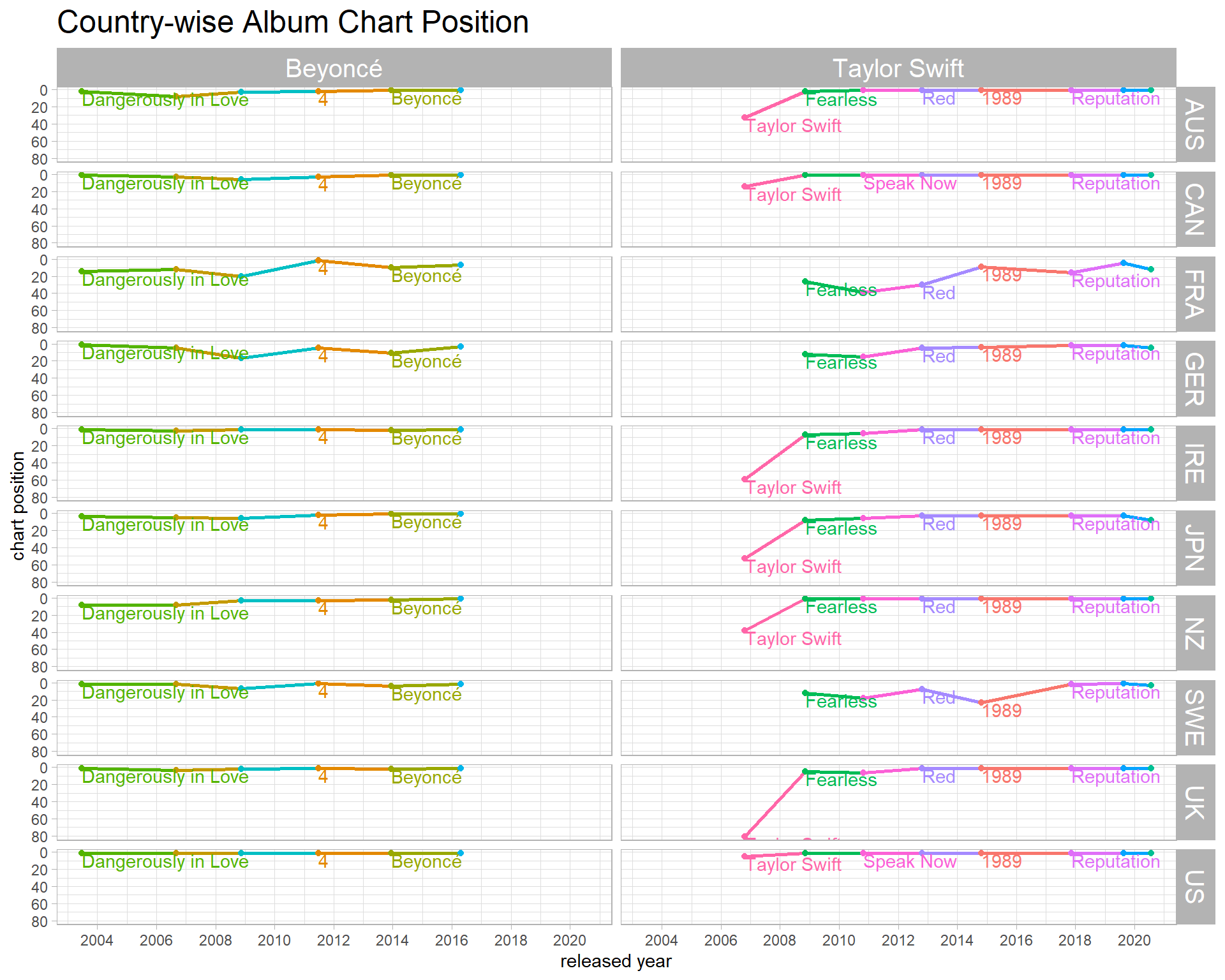
Album formats:
charts %>%
  separate_rows(formats, sep = ",\\s+") %>%
  group_by(artist, album, formats) %>%
  summarize(n = n()) %>%
  ungroup() %>%
  mutate(album = fct_reorder(album, n, sum)) %>%
  ggplot(aes(n, album, fill = formats)) +
  geom_col() +
  facet_wrap(~artist, scales = "free_y") +
  scale_x_continuous(breaks = seq(0, 80, 10)) +
  labs(x = "# of formats",
       fill = "format",
       title = "Albums Distribution Formats across Multiple Countries")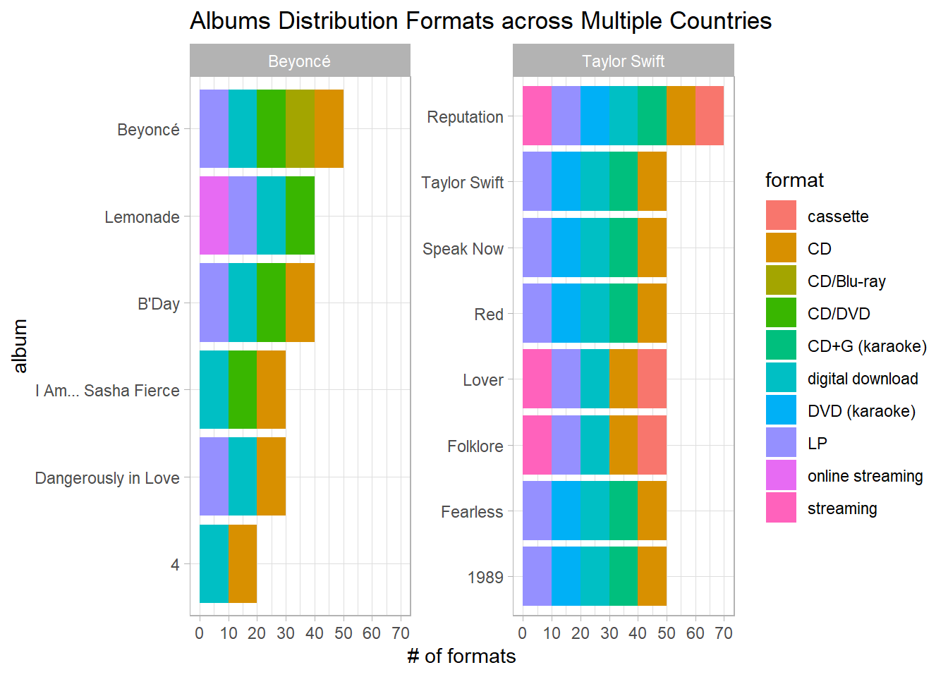
Working on sales:
sales %>%
  filter(country == "US") %>%
  mutate(title = fct_reorder(title, sales),
         artist = fct_reorder(artist, -sales, sum)) %>%
  ggplot(aes(sales, title, fill = artist)) +
  geom_col() +
  scale_x_continuous(labels = dollar) +
  labs(x = NULL,
       y = "album",
       fill = NULL,
       title = "Sales Volume per Album")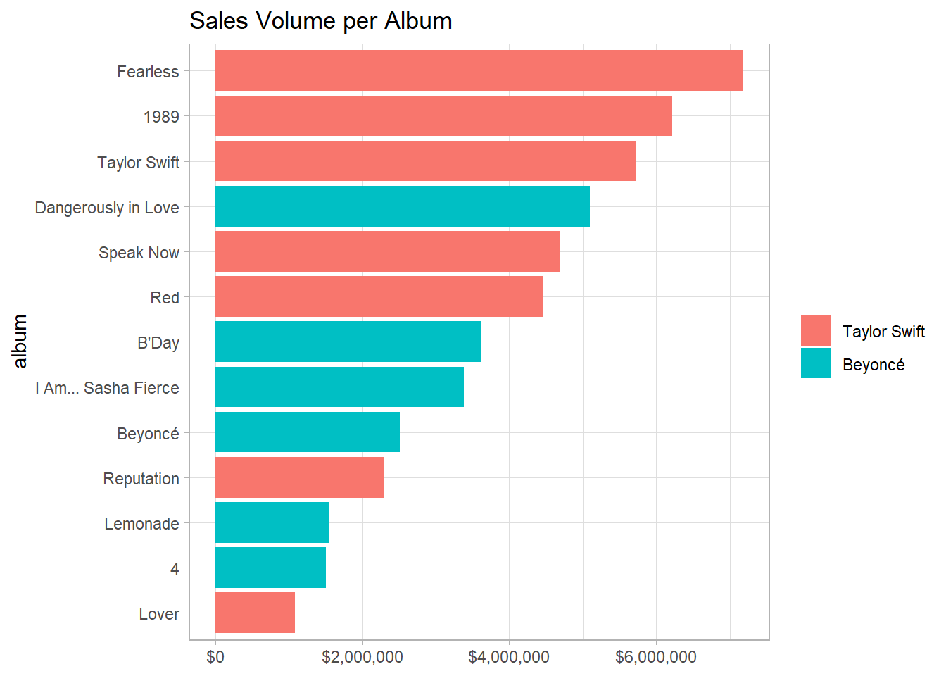
Working on taylor_swift_lyrics
Weighted log odds on Album words:
taylor_swift_lyrics %>%
  unnest_tokens(word, lyrics) %>%
  anti_join(stop_words) %>%
  count(album, word, sort = T) %>%
  bind_log_odds(album, word, n) %>%
  group_by(album) %>%
  slice_max(log_odds_weighted, n = 5) %>%
  ungroup() %>%
  mutate(word = reorder_within(word, log_odds_weighted, album)) %>%
  ggplot(aes(log_odds_weighted, word, fill = album)) +
  geom_col(show.legend = F) +
  scale_y_reordered() +
  facet_wrap(~album, scales = "free_y") +
  labs(x = "weighted log odds",
       y = NULL,
       title = "Top 5 Lyrics Words with the Largest Weighted Log Odds",
       subtitle = "For all ablums") +
  theme(strip.text = element_text(size = 15),
        plot.title = element_text(size = 17))
Weighted log odds on song words:
taylor_swift_lyrics %>%
  mutate(lyrics_length = str_length(lyrics)) %>%
  slice_max(lyrics_length, n = 9) %>%
  select(-lyrics_length) %>%
  unnest_tokens(word, lyrics) %>%
  anti_join(stop_words) %>%
  count(song, word, sort = T) %>%
  bind_log_odds(song, word, n) %>%
  group_by(song) %>%
  slice_max(log_odds_weighted, n = 5, with_ties = F) %>%
  ungroup() %>%
  mutate(word = reorder_within(word, log_odds_weighted, song),
         song = fct_reorder(song, -log_odds_weighted, sum)) %>%
  ggplot(aes(log_odds_weighted, word, fill = song)) +
  geom_col(show.legend = F) +
  scale_y_reordered() +
  facet_wrap(~song, scales = "free_y") +
  labs(x = "weighted log odds",
       y = NULL,
       title = "Top 5 Lyrics Words with the Largest Weighted Log Odds",
       subtitle = "For 9 most lengthy songs") +
  theme(strip.text = element_text(size = 13),
        plot.title = element_text(size = 17))
beyonce_lyrics analysis:
beyonce_processed <- beyonce_lyrics %>%
  distinct(line, .keep_all = T) %>%
  select(-contains("artist"))  %>%
  mutate(song_name = str_remove_all(song_name, "\\s?\\(.+$|\\s?\\[.+$")) %>%
  filter(song_id != 2985000)

beyonce_processed
## # A tibble: 10,791 x 4
## line song_id song_name song_line
## <chr> <dbl> <chr> <dbl>
## 1 If I ain't got nothing, I got you 50396 1+1 1
## 2 If I ain't got something, I don't give a damn 50396 1+1 2
## 3 'Cause I got it with you 50396 1+1 3
## 4 I don't know much about algebra, but I know 1+1 ~ 50396 1+1 4
## 5 And it's me and you 50396 1+1 5
## 6 That's all we'll have when the world is through 50396 1+1 6
## 7 'Cause baby, we ain't got nothing without love 50396 1+1 7
## 8 Darling, you got enough for the both of us 50396 1+1 8
## 9 So come on, baby, make love to me 50396 1+1 9
## 10 When my days look low 50396 1+1 10
## # ... with 10,781 more rowsbeyonce_processed has many same songs with various song_id, and the reason is these same songs have multiple versions (i.e., some are sung at studio, others at conference).
beyonce_joined <- beyonce_processed %>%
  inner_join(
    beyonce_processed %>%
      select(song_id, song_name) %>%
      distinct(song_name, .keep_all = T),
    by = c("song_name", "song_id")
)

beyonce_joined
## # A tibble: 8,701 x 4
## line song_id song_name song_line
## <chr> <dbl> <chr> <dbl>
## 1 If I ain't got nothing, I got you 50396 1+1 1
## 2 If I ain't got something, I don't give a damn 50396 1+1 2
## 3 'Cause I got it with you 50396 1+1 3
## 4 I don't know much about algebra, but I know 1+1 ~ 50396 1+1 4
## 5 And it's me and you 50396 1+1 5
## 6 That's all we'll have when the world is through 50396 1+1 6
## 7 'Cause baby, we ain't got nothing without love 50396 1+1 7
## 8 Darling, you got enough for the both of us 50396 1+1 8
## 9 So come on, baby, make love to me 50396 1+1 9
## 10 When my days look low 50396 1+1 10
## # ... with 8,691 more rowsbeyonce_joined only contains each song with one unique song_id.
beyonce_joined %>%
  distinct(song_name, song_id) %>%
  count(song_name, sort = T)
## # A tibble: 259 x 2
## song_name n
## <chr> <int>
## 1 "\"Self-Titled\" Part 1 . The Visual Album" 1
## 2 "\"Self-Titled\" Part 2 . Imperfection" 1
## 3 "***Flawless" 1
## 4 "<U+200B>come home" 1
## 5 "<U+200B>war" 1
## 6 "<U+200E>blind trust" 1
## 7 "1+1" 1
## 8 "6 Inch" 1
## 9 "7/11" 1
## 10 "A Woman Like Me" 1
## # ... with 249 more rowsNow we can see confirm it.
Sentiment analysis:
beyonce_joined %>%
  unnest_tokens(word, line) %>%
  anti_join(stop_words) %>%
  inner_join(get_sentiments("afinn"), by = "word") %>%
  group_by(song_name) %>%
  summarize(value = mean(value)) %>%
  ungroup() %>%
  group_by(value > 0) %>%
  slice_max(abs(value), n = 5, with_ties = F) %>%
  ungroup() %>%
  mutate(song_name = fct_reorder(song_name, value)) %>%
  ggplot(aes(value, song_name, fill = value > 0)) +
  geom_col() +
  theme(legend.position = "none") +
  labs(x = "AFINN mean value",
       y = NULL,
       title = "The 5 Happiest and Saddest Beyonce Songs based on AFINN")