Data Visualization on the Great American Beer Festival (Logistic Regression Used)
Sat, Feb 26, 2022
5-minute read
The data for this blog post is from TidyTuesday.
library(tidyverse)
library(geofacet)
library(tidytext)
library(tidylo)
library(scales)
library(broom)
theme_set(theme_light())
beer_awards <- read_csv('https://raw.githubusercontent.com/rfordatascience/tidytuesday/master/data/2020/2020-10-20/beer_awards.csv') %>%
mutate(state = str_to_upper(state),
medal = factor(medal, levels = c("Bronze", "Silver", "Gold")))
beer_awards## # A tibble: 4,970 x 7
## medal beer_name brewery city state category year
## <fct> <chr> <chr> <chr> <chr> <chr> <dbl>
## 1 Gold Volksbier Vienna Wibby ~ Long~ CO America~ 2020
## 2 Silver Oktoberfest Founde~ Gran~ MI America~ 2020
## 3 Bronze Amber Lager Skippi~ Stau~ VA America~ 2020
## 4 Gold Lager at World's End Epidem~ Conc~ CA America~ 2020
## 5 Silver Seismic Tremor Seismi~ Sant~ CA America~ 2020
## 6 Bronze Lite Thinking Pollya~ Lemo~ IL America~ 2020
## 7 Gold Beachscape Ventur~ Vent~ CA America~ 2020
## 8 Silver Imagine a World with Beer Cellars ~ Freeta~ San ~ TX America~ 2020
## 9 Bronze Pilsner Old To~ Port~ OR America~ 2020
## 10 Gold Tank 7 Boulev~ Kans~ MO America~ 2020
## # ... with 4,960 more rowsMedal counts:
beer_awards %>%
  count(year, state, medal, sort = T) %>%
  ggplot(aes(year, n, color = medal)) +
  geom_line(size = 1) +
  facet_geo(~state) +
  theme(strip.text = element_text(size = 15),
        plot.title = element_text(size = 18)) +
  labs(y = "# of medals",
title = "State-wise Medal Counts across Years") 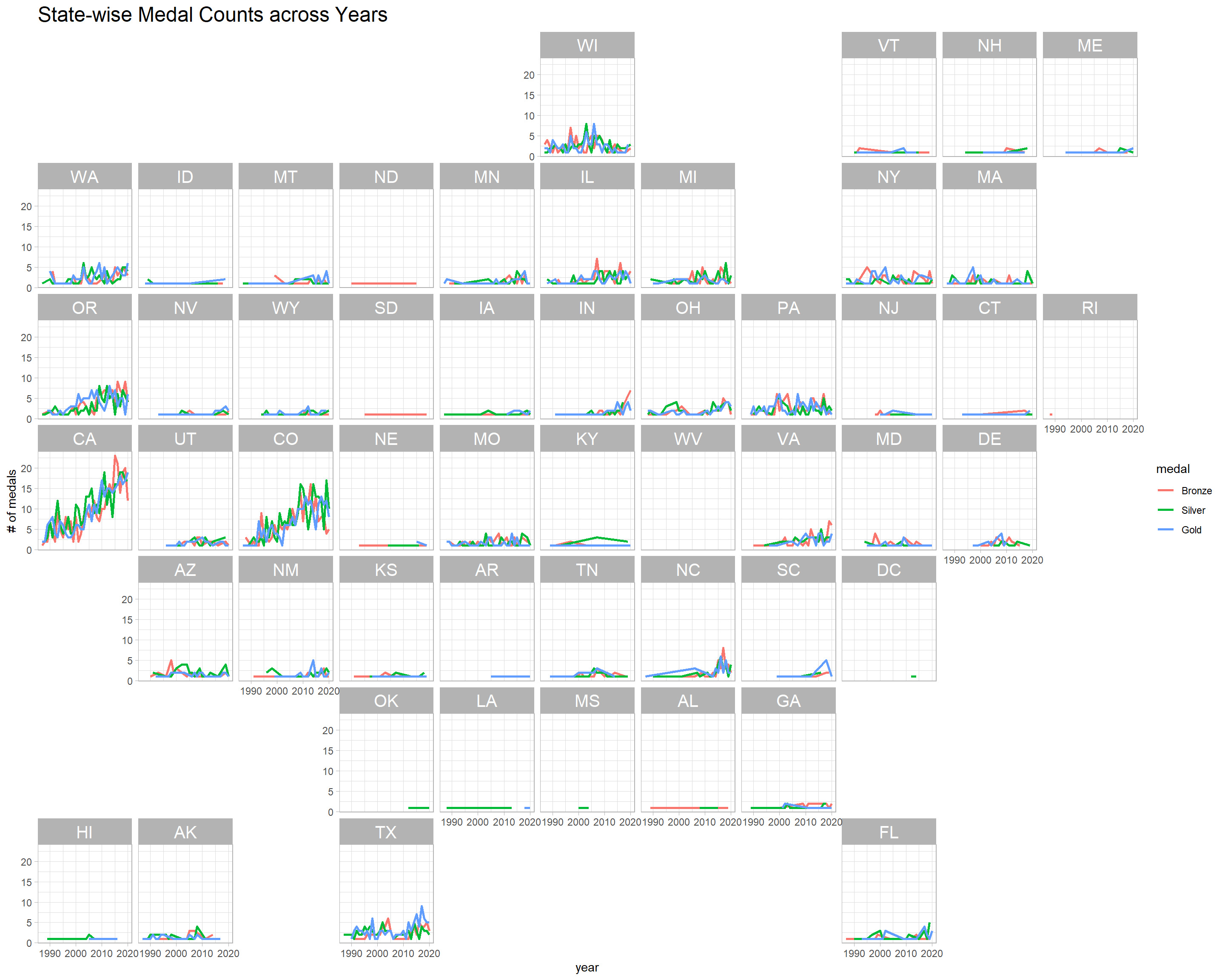
Gold beers:
beer_awards %>%
  filter(medal == "Gold") %>%
  group_by(beer_name, state) %>%
  summarize(year_min = min(year),
            year_max = max(year),
            year_diff = year_max - year_min,
            n = n()) %>%
  arrange(desc(year_diff)) %>%
  filter(n > 2) %>%
  ungroup() %>%
  ggplot(aes(year_min, year_max, color = state)) +
  geom_point(aes(size = n)) +
  geom_text(aes(label = beer_name), check_overlap = T, hjust = 1, vjust = 1) +
  labs(x = "first year getting gold medal",
       y = "last year getting gold medal",
       size = "# of gold medals",
title = "Gold-medal Beers with Respect to Year and State") 
Top 8 beer categories:
beer_awards %>%
  count(category, medal, sort = T) %>%
  group_by(medal) %>%
  slice_max(n, n = 8, with_ties = F) %>%
  ungroup() %>%
  mutate(category = fct_reorder(category, n, sum)) %>%
  ggplot(aes(n, category, fill = medal)) +
  geom_col() +
  labs(x = "# of medals",
       y = "beer category",
       fill = NULL,
title = "Top 8 Categories per Medal") 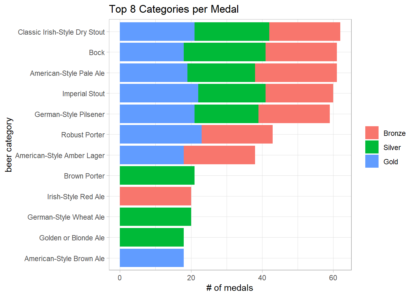
Which city is famous for beer and brewery?
beer_awards %>%
  count(state, city, medal, sort = T) %>%
  head(100) %>%
  mutate(city = paste0(city, " (", state, ")")) %>%
  mutate(city = reorder_within(city, n, medal)) %>%
  ggplot(aes(n, city, fill = medal)) +
  geom_col() +
  scale_y_reordered() +
  facet_wrap(~medal, scales = "free_y") +
  theme(legend.position = "none",
        strip.text = element_text(size = 15),
        plot.title = element_text(size = 18)) +
  labs(x = "# of awards",
       y = "city with state",
       title = "Which City is the Most Beer-awarded City?")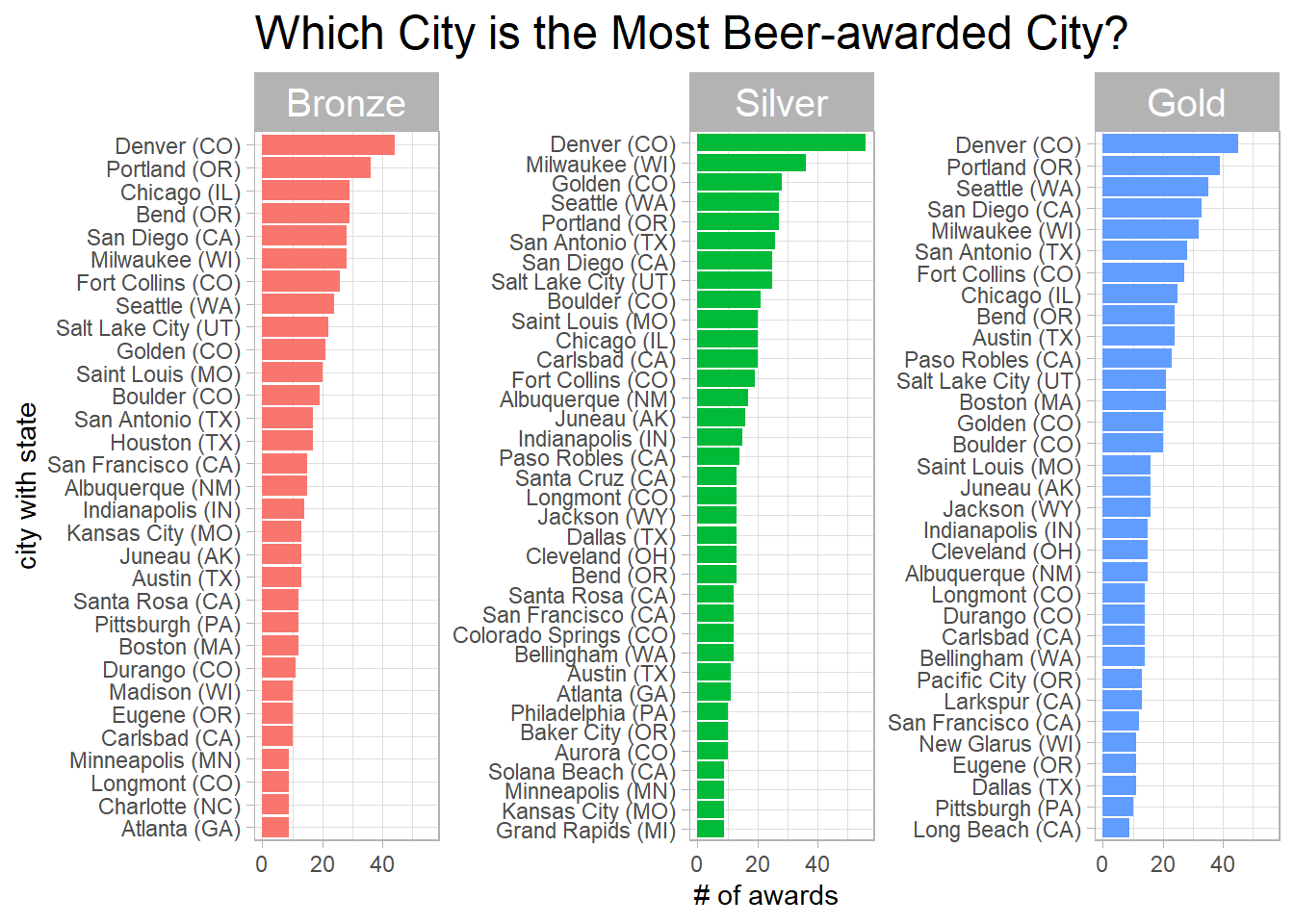
Top 10 Breweries:
beer_awards %>%
  filter(fct_lump(brewery, n = 10) != "Other") %>%
  count(brewery, medal, sort = T) %>%
  mutate(brewery = fct_reorder(brewery, n, sum)) %>%
  ggplot(aes(medal, brewery, fill = n)) +
  geom_tile() +
  scale_fill_gradient2(high = "green",
                       low = "red",
                       midpoint = 15) +
  scale_x_discrete(expand = c(0,0)) +
  scale_y_discrete(expand = c(0,0)) +
  labs(x = NULL,
       y = NULL,
       fill = "# of medals",
       title = "10 Most-awarded Breweries and Their Medal Counts") +
  theme(plot.title = element_text(size = 18),
        axis.text = element_text(size = 13))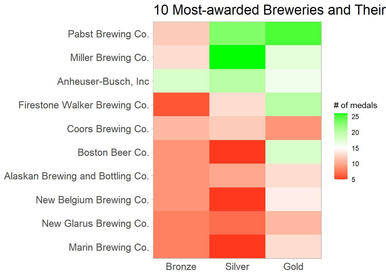
beer_joined <- beer_awards %>%
  count(beer_name, medal, brewery, sort = T) %>%
  group_by(beer_name, brewery) %>%
  summarize(n = n()) %>%
  filter(n > 1) %>%
  ungroup() %>%
  select(-n) %>%
  inner_join(beer_awards,
             by = c("beer_name", "brewery"))

beer_joined
## # A tibble: 1,003 x 7
## beer_name brewery medal city state category year
## <chr> <chr> <fct> <chr> <chr> <chr> <dbl>
## 1 2004 Triple Exultation Eel River Brewing C~ Silv~ Fort~ CA Aged Be~ 2012
## 2 2004 Triple Exultation Eel River Brewing C~ Bron~ Fort~ CA Aged Be~ 2011
## 3 5 Barrel Pale Ale Odell Brewing Co. Gold Fort~ CO Classic~ 2013
## 4 5 Barrel Pale Ale Odell Brewing Co. Silv~ Fort~ CO Classic~ 2005
## 5 Abbey Belgian Style Ale New Belgium Brewing~ Bron~ Fort~ CO Belgian~ 2005
## 6 Abbey Belgian Style Ale New Belgium Brewing~ Gold Fort~ CO Belgian~ 2004
## 7 Abbey Belgian Style Ale New Belgium Brewing~ Gold Fort~ CO Belgian~ 2003
## 8 Abbey Belgian Style Ale New Belgium Brewing~ Bron~ Fort~ CO Belgian~ 2001
## 9 Abbey Belgian Style Ale New Belgium Brewing~ Gold Fort~ CO Belgian~ 2000
## 10 Abbey Belgian Style Ale New Belgium Brewing~ Bron~ Fort~ CO Belgian~ 1998
## # ... with 993 more rowsWhich beers fluctuated the medals?
beer_joined %>%
  filter(fct_lump(beer_name, n = 9) != "Other") %>%
  ggplot(aes(year, medal, color = beer_name, group = beer_name)) +
  geom_line(size = 1) +
  geom_point() +
  facet_wrap(~beer_name) +
  theme(legend.position = "none",
        strip.text = element_text(size = 11),
        plot.title = element_text(size = 18)) +
  labs(y = NULL,
       title = "Beers that Fluctuated among the Medals?")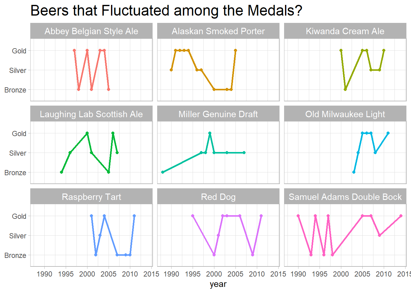
The following code snippets are inspired by David Robinson. Here you can find his code.
Which beer category is over represented per state?
beer_awards %>%
  mutate(state = state.name[match(state, state.abb)]) %>%
  filter(fct_lump(state, n = 9) != "Other",
         fct_lump(category, n = 12) != "Other") %>%
  count(category, state, sort = T) %>%
  complete(state, category, fill = list(n = 0)) %>%
  bind_log_odds(state, category, n) %>%
  mutate(category = reorder_within(category, log_odds_weighted, state)) %>%
  ggplot(aes(log_odds_weighted, category, fill = log_odds_weighted > 0)) +
  geom_col() +
  scale_y_reordered() +
  facet_wrap(~state, scales = "free_y") +
  theme(legend.position = "none",
        strip.text = element_text(size = 15),
        plot.title = element_text(size = 18)) +
  labs(x = "weighted log odds",
       y = "beer category",
       title = "Which Beer Category is Over or Under Represented?")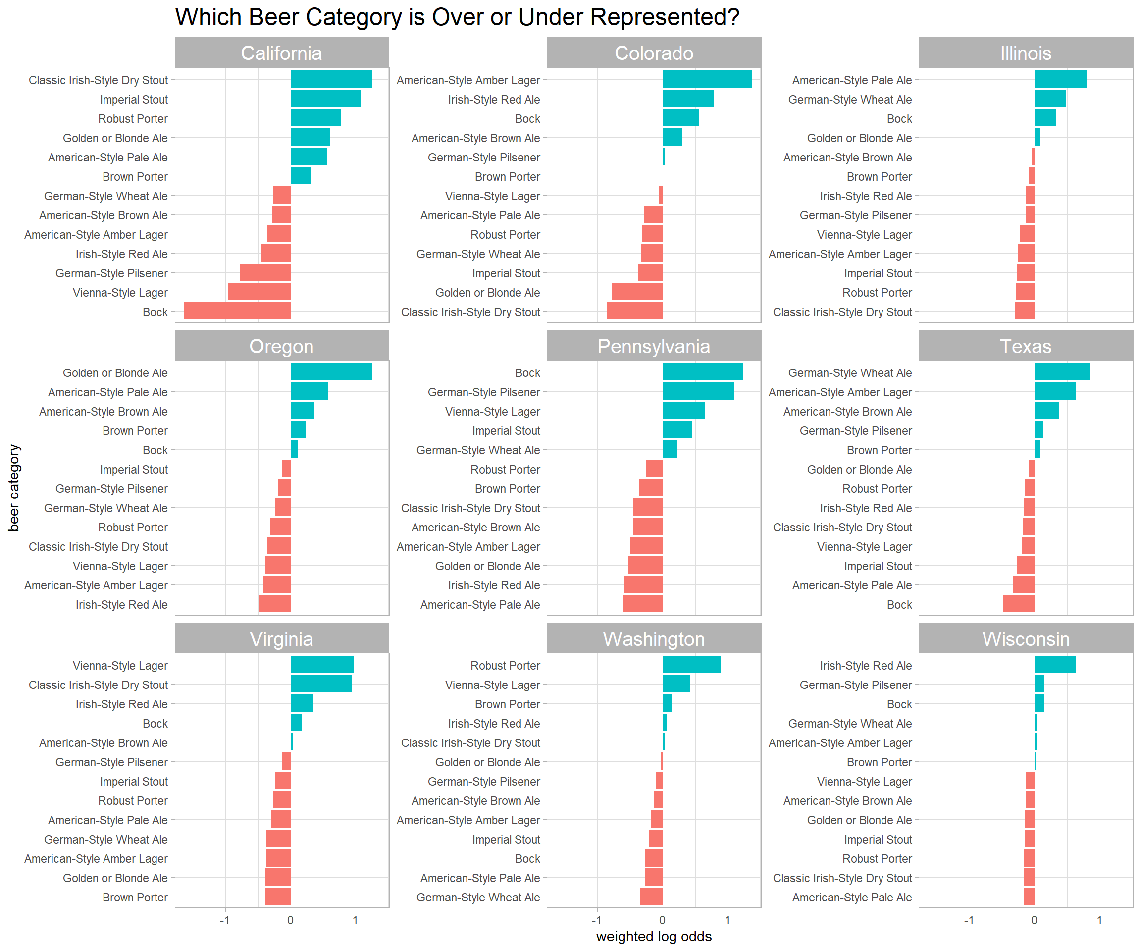
by_year <- beer_awards %>%
  add_count(year, name = "year_total") %>%
  mutate(state = fct_lump(state, n = 9)) %>%
  filter(state != "Other") %>%
  count(state, year, year_total, sort = T) %>%
  mutate(pct_year = n/year_total)

by_year %>%
  ggplot(aes(year, pct_year, color = state)) +
  geom_line(size = 1) +
  expand_limits(y = 0) +
  scale_y_continuous(labels = percent) +
facet_wrap(~ state) 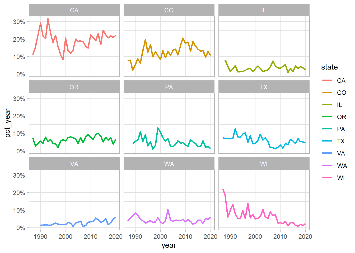
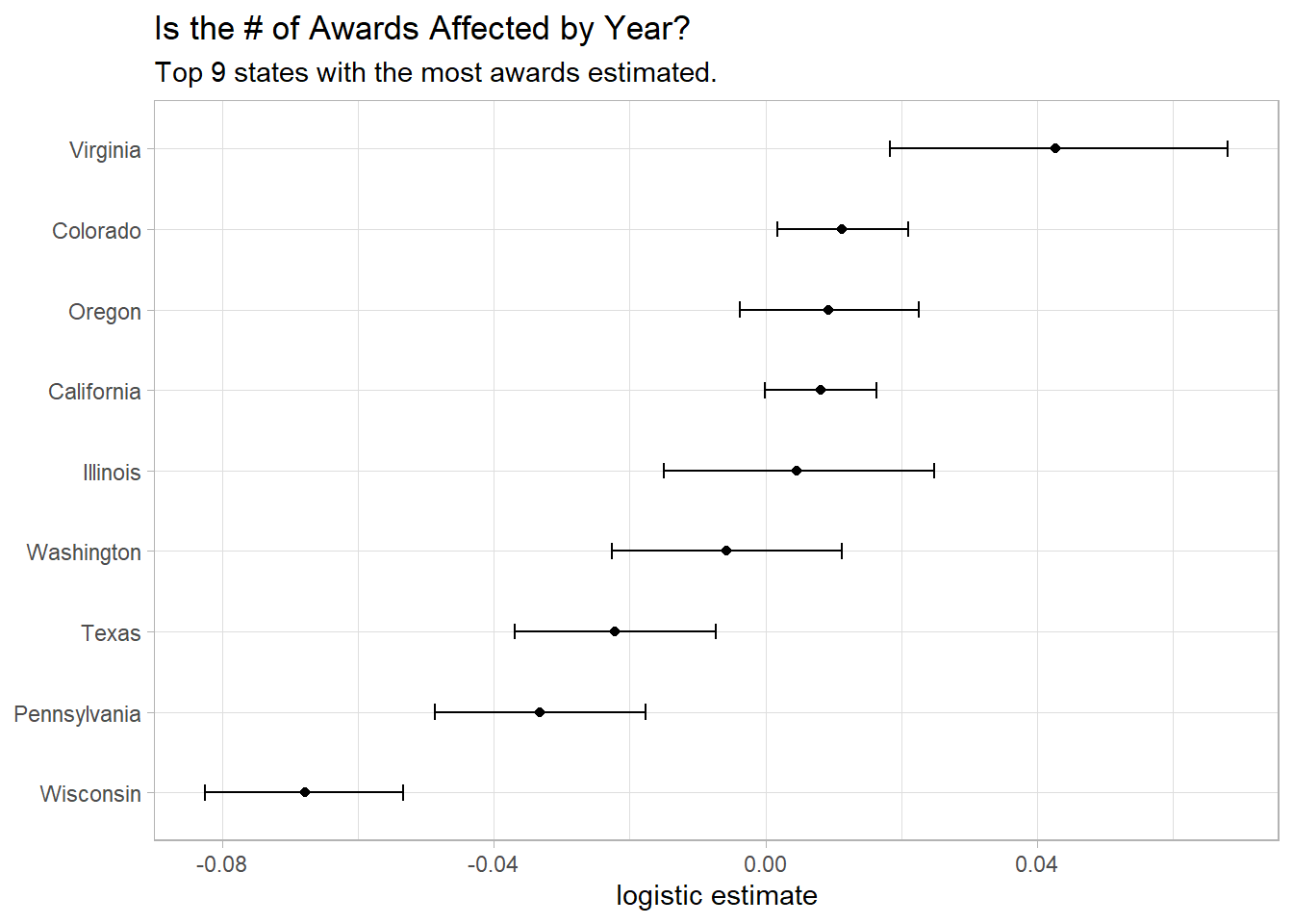
by_year %>%
  mutate(state = state.name[match(state, state.abb)]) %>%
  group_by(state) %>%
  summarize(model = list(glm(cbind(n, year_total - n) ~ year, family = "binomial"))) %>%
  mutate(tidied = map(model, tidy, conf.int = T)) %>%
  unnest(tidied) %>%
  filter(term == "year") %>%
  mutate(p.value = format.pval(p.value),
         state = fct_reorder(state, estimate)) %>%
  ggplot(aes(estimate, state)) +
  geom_point() +
  geom_errorbarh(aes(xmin = conf.low,
                     xmax = conf.high),
                 height = 0.2) +
  labs(x = "logistic estimate",
       y = NULL,
       title = "Is the # of Awards Affected by Year?",
       subtitle = "Top 9 states with the most awards estimated.")