IKEA Visualization & Modeling

This blog post analyzes the IKEA dataset from TidyTuesday.

library(tidyverse)
library(tidylo)
library(tidytext)
library(scales)
library(widyr)
library(ggraph)
theme_set(theme_light())

ikea <- read_csv('https://raw.githubusercontent.com/rfordatascience/tidytuesday/master/data/2020/2020-11-03/ikea.csv') %>%
  select(-1) %>%
  mutate(name = str_to_title(name),
         old_price = if_else(old_price == "No old price", price, parse_number(old_price)))

The typical furniture names per category:

ikea %>%
  count(name, category, sort = T) %>%
  bind_log_odds(category, name, n) %>%
  group_by(category) %>%
  slice_max(log_odds_weighted, n = 10, with_ties = F) %>%
  ungroup() %>%
  mutate(name = reorder_within(name, log_odds_weighted, category)) %>%
  ggplot(aes(log_odds_weighted, name, fill = category)) +
  geom_col() +
  scale_y_reordered() +
  facet_wrap(~category, scales = "free_y") +
  theme(legend.position = "none") +
  labs(x = "weighted log odds",
       y = "furniture name",
       title = "Top 10 Most Represented Names per Furniture Category")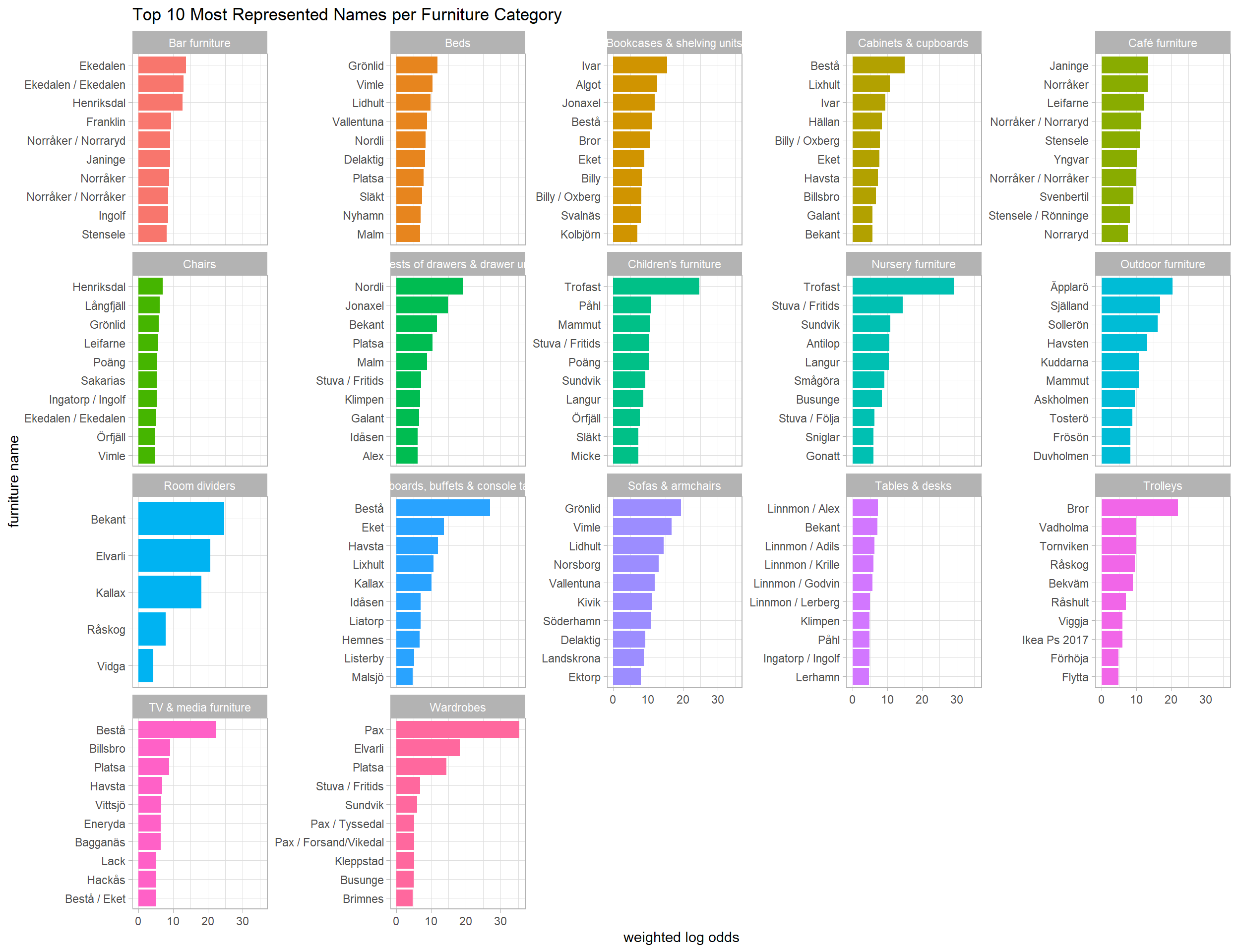 

Sellable online?

ikea %>%
  count(category, sellable_online, sort = T) %>% 
  mutate(category = fct_reorder(category, n, sum)) %>%
  ggplot(aes(n, category, fill = sellable_online)) +
  geom_col() +
  labs(x = "# of items",
       y = "",
       fill = "sellable online?",
       title = "Can All Items be Sold Online?")

Now let’s look close on what makes the items not sellable online.

ikea %>%
  ggplot(aes(price, fill = sellable_online)) +
  geom_histogram() +
  scale_x_continuous(label = dollar)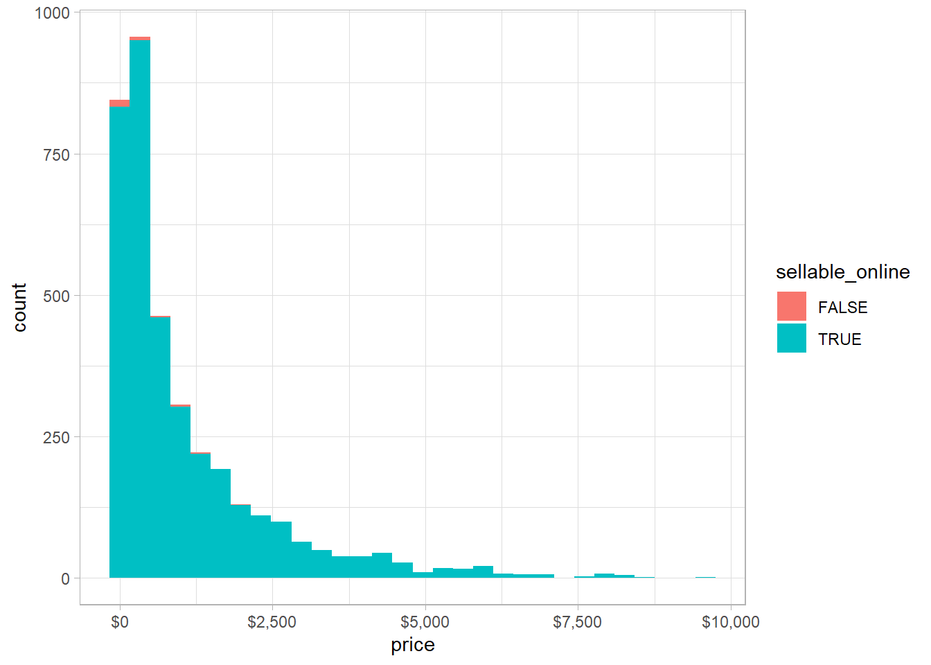

There are just few items that are not sellable online, and the price of these items varies, but on the lower end.

The most disounted items:

ikea %>%
  mutate(discount = old_price - price) %>%
  filter(discount > 0) %>% 
  group_by(category) %>%
  slice_max(discount, n = 10) %>%
  ungroup() %>%
  ggplot(aes(old_price, price, color = category)) +
  geom_point(aes(size = discount)) +
  geom_text(aes(label = paste0(name, "($", discount, ")")), 
            check_overlap = T,
            hjust = 1, 
            vjust = 1) +
  scale_size_continuous(guide = "none") +
  labs(x = "price before disount",
       y = "price after discount",
       title = "Top 10 Discounted Items per Category",
       subtitle = "Item names and discount $ are shown as text") +
  coord_fixed() +
  theme(panel.grid = element_blank())

The more higher the item price is, the more discount it enjoys.

Which category is the most expensive category?

ikea %>%
  mutate(category = fct_reorder(category, price)) %>%
  ggplot(aes(price, category, fill = category)) +
  geom_boxplot(show.legend = F) +
  scale_x_log10(label = dollar) +
  labs(x = NULL,
       title = "Furniture Pricing per Category")

It seems like TV & media furniture is the lowest category on pricing, but the Wardrobes category is the highest one.

Linear regression on price being predicted by detph, height, and width:

ikea %>%
  group_by(category) %>%
  summarize(model = list(lm(price ~ depth + height + width)),
            tidied = map(model, tidy, conf.int = T)) %>%
  unnest(tidied) %>%
  filter(term != "(Intercept)") %>%
  mutate(category = reorder_within(category, estimate, term)) %>%
  ggplot(aes(estimate, category, color = term)) +
  geom_point() +
  geom_vline(xintercept = 0, lty = 2) +
  geom_errorbarh(aes(xmin = conf.low, xmax = conf.high), height = 0.2) +
  facet_wrap(~term, scales = "free_y") +
  scale_y_reordered() +
  theme(legend.position = "none",
        strip.text = element_text(size = 15),
        plot.title = element_text(size = 18)) +
  labs(x = "linear regression estimate",
       title = "How does Furniture Dimension Affect Price?",
       subtitle = "The error bars represent 95% of CI")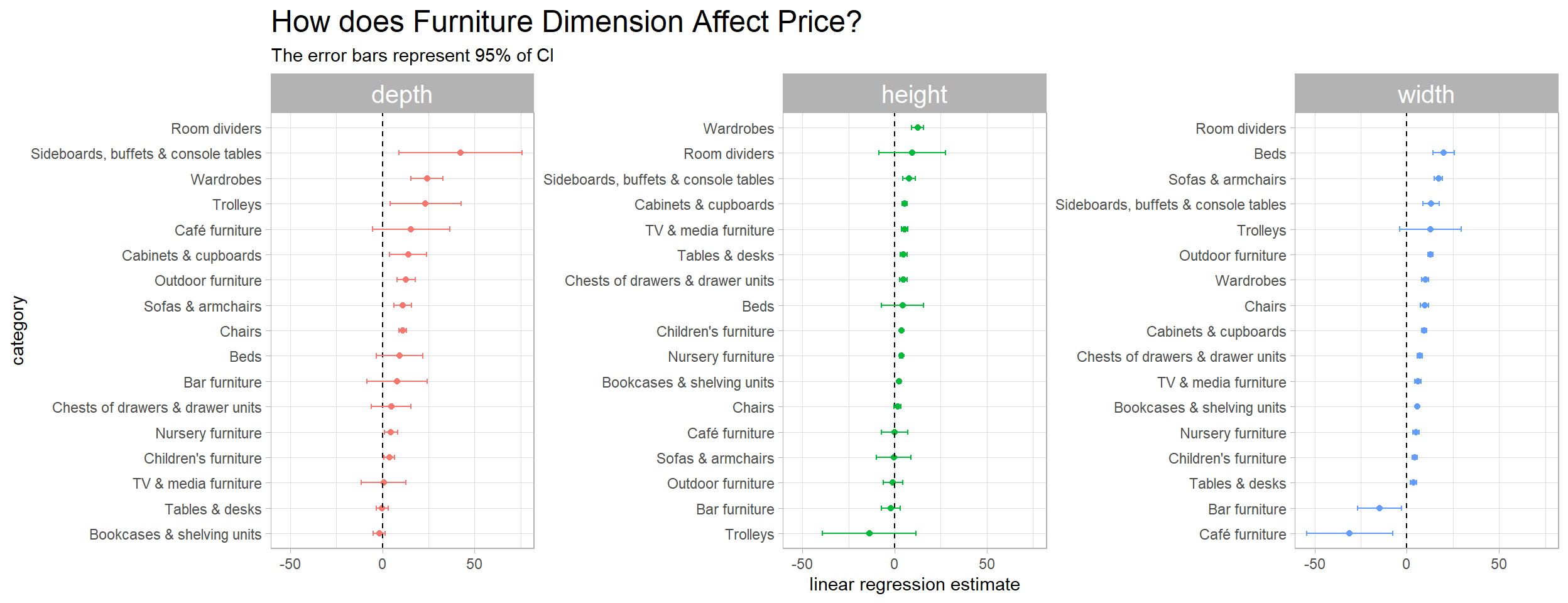 

set.seed(2022)
ikea %>%
  filter(fct_lump(designer, n = 10) != "Other") %>%
  count(designer, category, sort = T) %>%
  pairwise_cor(designer, category, n) %>%
  ggraph(layout = "fr") +
  geom_edge_link(aes(width = correlation),
                 alpha = 0.3,
                 color = "lightblue") +
  geom_node_point() +
  geom_node_text(aes(label = name), vjust = 1, hjust = 0, check_overlap = T) +
  scale_edge_width_continuous(range = c(1,3)) +
  ggtitle("How Correlated of Designers within Category?",
          subtitle = "Top 10 desingers are chosen.")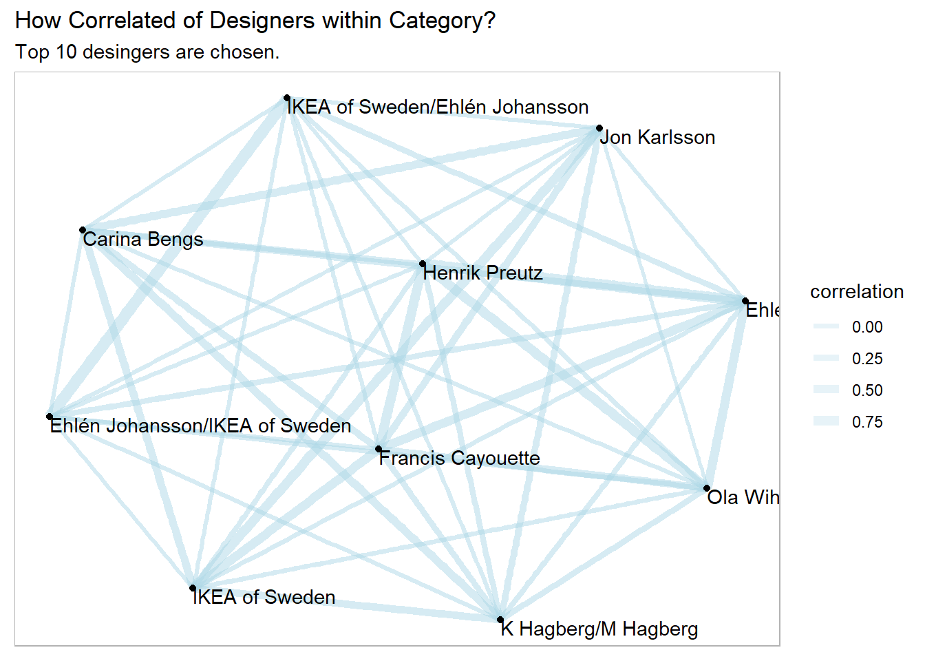 

ikea %>%
  count(other_colors, category, sort = T) %>%
  pivot_wider(names_from = other_colors,
              values_from = n) %>%
  mutate(total = Yes + No,
         pct_colors = Yes/total,
         category = fct_reorder(category, pct_colors)) %>%
  ggplot(aes(pct_colors, category)) +
  geom_point(aes(size = total), color = "#ffcc00") +
  scale_x_continuous(labels = percent) +
  scale_size_continuous(breaks = seq(100, 600, 100)) +
  labs(x = "% of furniture having multiple colors",
       y = NULL,
       size = "total # of items",
       title = "Category-wise Furniture with Multiple Colors")