Ninja Warrior Data Visualization

In this blog post, I would like to analyze the Ninja Warrior data from TidyTuesday. I need to claim I know nothing about the show, and this is a perfect opportunity to investigate the data without any background information. The data is relatively simple.

library(tidyverse)
library(tidylo)
theme_set(theme_light())

warrior <- read_csv('https://raw.githubusercontent.com/rfordatascience/tidytuesday/master/data/2020/2020-12-15/ninja_warrior.csv') %>%
  mutate(round_stage = str_remove(round_stage, "\\s\\(Regional/City\\)"),
         round_stage = factor(round_stage, levels = c("Qualifying",
                                                      "Semi-Finals",
                                                      "National Finals - Stage 1",
                                                      "National Finals - Stage 2",
                                                      "National Finals - Stage 3",
                                                      "National Finals - Stage 4",
                                                      "Finals")))


warrior

## # A tibble: 889 x 5
##    season location round_stage obstacle_name   obstacle_order
##     <dbl> <chr>    <fct>       <chr>                    <dbl>
##  1      1 Venice   Qualifying  Quintuple Steps              1
##  2      1 Venice   Qualifying  Rope Swing                   2
##  3      1 Venice   Qualifying  Rolling Barrel               3
##  4      1 Venice   Qualifying  Jumping Spider               4
##  5      1 Venice   Qualifying  Pipe Slider                  5
##  6      1 Venice   Qualifying  Warped Wall                  6
##  7      1 Venice   Semi-Finals Quintuple Steps              1
##  8      1 Venice   Semi-Finals Rope Swing                   2
##  9      1 Venice   Semi-Finals Rolling Barrel               3
## 10      1 Venice   Semi-Finals Jumping Spider               4
## # ... with 879 more rows

Season and round stages:

warrior %>%
  count(season, round_stage) %>%
  mutate(season = paste("Season", season),
         season = fct_reorder(season, parse_number(season))) %>%
  ggplot(aes(n, season, fill = round_stage)) +
  geom_col() +
  labs(x = "# of season rounds",
       y = NULL,
       fill = NULL,
       title = "# of Rounds per Season")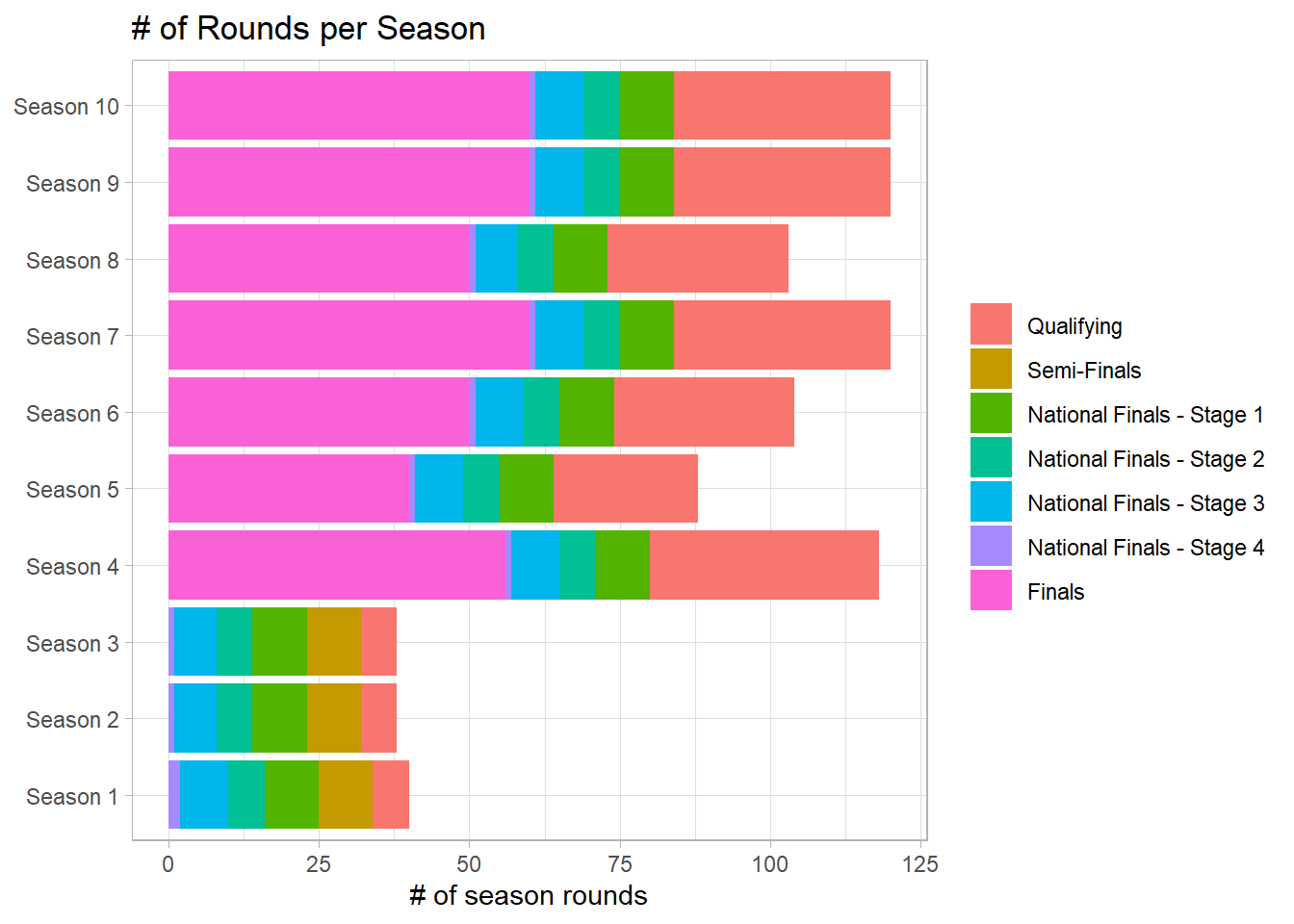

warrior %>%
  group_by(season, round_stage) %>%
  summarize(n = n_distinct(obstacle_order)) %>% 
  ungroup() %>%
  ggplot(aes(factor(season), round_stage, fill = n)) +
  geom_tile() +
  labs(x = "season",
       y = NULL,
       fill = "# of rounds",
       title = "Season and Round State Count") +
  scale_fill_gradient2(high = "green",
                       low = "red",
                       midpoint = 5,
                       breaks = seq(1,10,2)) +
  theme(panel.grid = element_blank())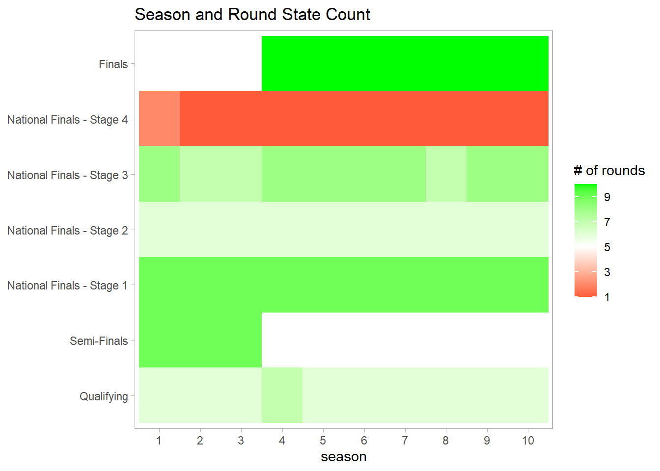

The first four seasons do not have finals.

Does each season have its favorite place?

warrior %>%
  count(season, location, sort = T) %>%
  bind_log_odds(season, location, n) %>%
  mutate(location = fct_reorder(location, log_odds_weighted, sum)) %>%
  ggplot(aes(log_odds_weighted, location, fill = factor(season))) +
  geom_col() +
  labs(x = "weighted log odds",
       y = "",
       fill = "season",
       title = "Which Season is of Speciality to Location?",
       subtitle = "The speciality is measured by weighted log odds.")

The easiest and hardest obstacle of each round:

warrior %>%
  group_by(round_stage) %>%
  slice_max(obstacle_order, n = 1) %>%
  ungroup() %>%
  count(obstacle_name, sort = T) %>%
  mutate(difficulty = "hard") %>%
  bind_rows(warrior %>%
              group_by(round_stage) %>%
              slice_min(obstacle_order, n = 1) %>%
              ungroup() %>%
              count(obstacle_name, sort = T) %>%
              mutate(difficulty = "easy",
                     n = -n)) %>% 
  mutate(obstacle_name = fct_reorder(obstacle_name, n)) %>%
  ggplot(aes(n, obstacle_name, fill = difficulty)) +
  geom_col() +
  scale_x_continuous(labels = function(x) abs(x)) +
  labs(x = "# of times this obstacle appears",
       y = "obstacle",
       title = "Which Obstacle is More Likely to be Easiest or Hardest?")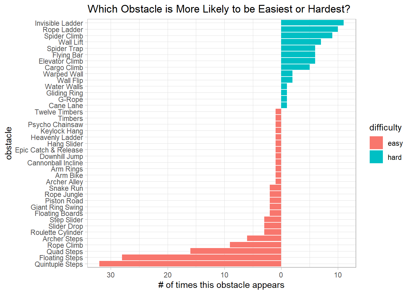

It seems like the Quintuple Steps is the most adopted easiest obstacle in the show, and its hardest counterpart is the Invisible Ladder. I guess it is invisible, thus making it hard.

warrior %>%
  mutate(obstacle_name = fct_lump(obstacle_name, n = 10, ties.method = "first"),
         obstacle_name = fct_reorder(obstacle_name, obstacle_order)) %>%
  ggplot(aes(obstacle_order, obstacle_name)) +
  geom_boxplot() +
  scale_x_continuous(breaks = seq(1,10)) +
  labs(x = "obstacle order",
       y = "obstacle",
       title = "10 Most Popular Obstacles and Their Respective Order")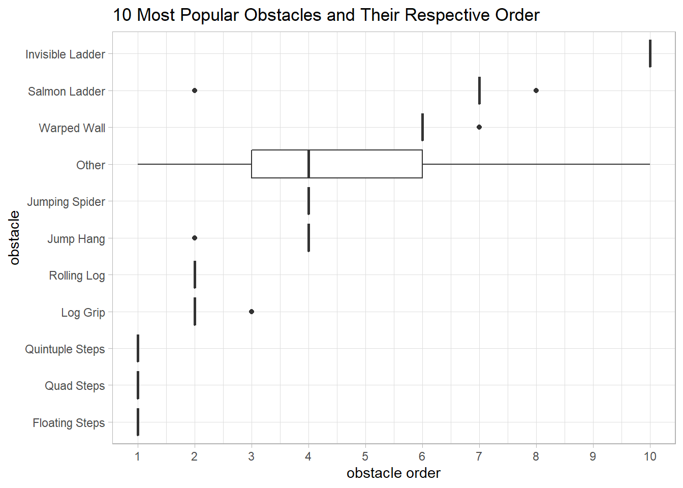

What is surprising is that almost all 10 popular obstacles do not fluctuate on their order much, at most 1 order difference.

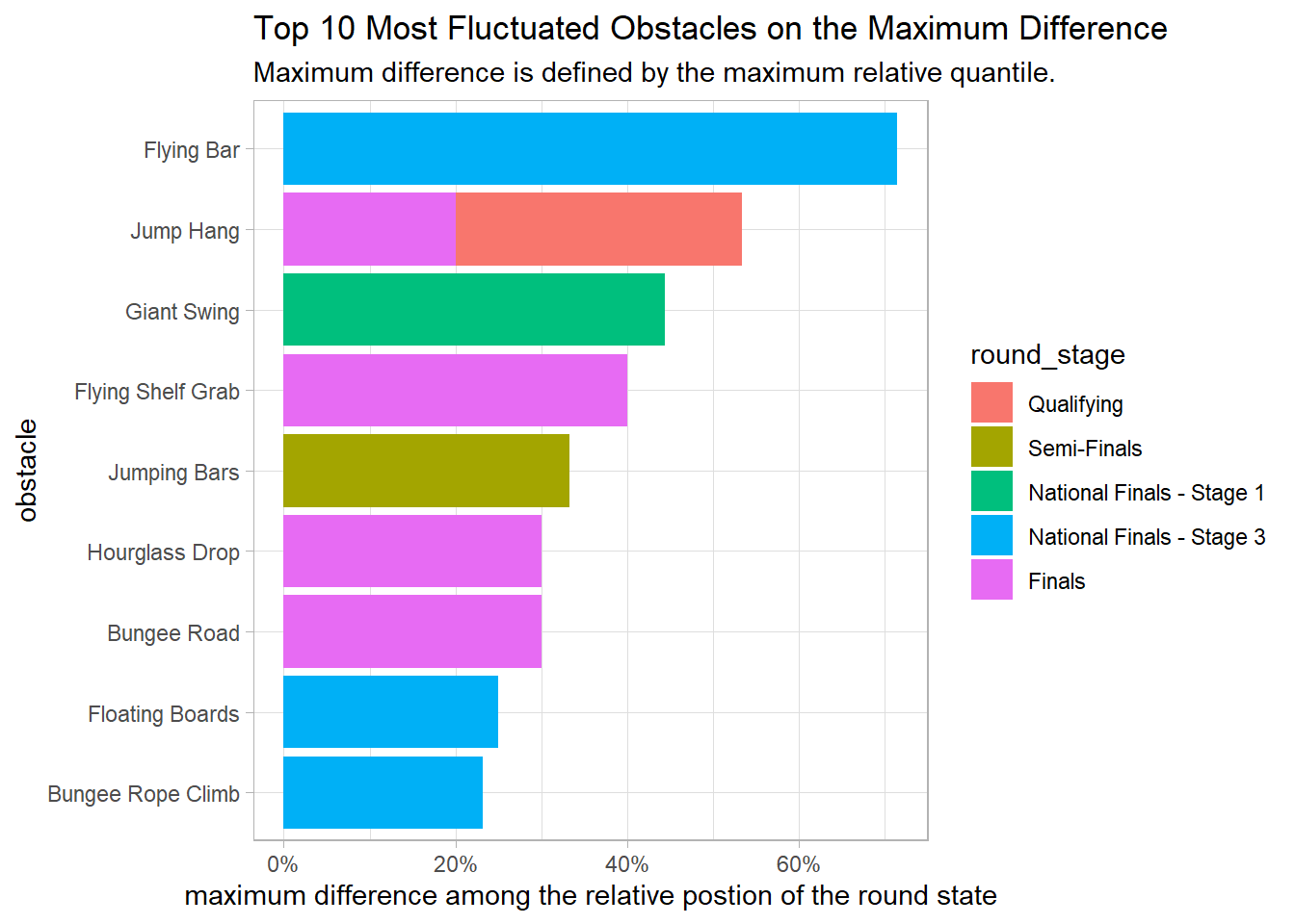
Based on the plot above, it is intriguing to investigate which obstacles do change with respect to their relative position at various round stages.

warrior %>%
  group_by(season, round_stage) %>%
  mutate(order_quantile = obstacle_order/max(obstacle_order)) %>%
  group_by(obstacle_name, round_stage) %>%
  summarize(order_diff = max(order_quantile) - min(order_quantile),
            n = n()) %>%
  arrange(desc(order_diff)) %>% 
  head(10) %>%
  ungroup() %>%
  mutate(obstacle_name = fct_reorder(obstacle_name, order_diff, sum)) %>%
  ggplot(aes(order_diff, obstacle_name, fill = round_stage)) +
  geom_col() +
  scale_x_continuous(labels = scales::percent) +
  labs(x = "maximum difference among the relative postion of the round state",
       y = "obstacle",
       title = "Top 10 Most Fluctuated Obstacles on the Maximum Difference",
       subtitle = "Maximum difference is defined by the maximum relative quantile.")