Data Visualization on Transit Costs
Fri, Mar 4, 2022
4-minute read
In this blog post, I will analyze the cost associated with the transit projects each country spends on. The data comes from TidyTuesday.
library(tidyverse)
library(countrycode)
library(scales)
library(patchwork)
theme_set(theme_light())
Read the data and process it by renaming some columns and adding new ones.
transit_cost <- read_csv('https://raw.githubusercontent.com/rfordatascience/tidytuesday/master/data/2021/2021-01-05/transit_cost.csv') %>%
  distinct() %>%
  filter(length < 2500) %>%
  rename(id = e,
         railway = rr,
         length_completed = tunnel,
         cost_usd = real_cost,
         cost_km_usd = cost_km_millions) %>%
  mutate(across(5:6, as.numeric),
         project_duration = end_year - start_year + 1,
         cost_usd = as.numeric(cost_usd),
         country = fct_recode(country, "GB" = "UK"),
         country_name = countrycode(country, origin = "iso2c", destination = "country.name"))

transit_cost
## # A tibble: 535 x 22
## id country city line start_year end_year railway length tunnel_per
## <dbl> <fct> <chr> <chr> <dbl> <dbl> <dbl> <dbl> <chr>
## 1 7136 CA Vancouver Broa~ 2020 2025 0 5.7 87.72%
## 2 7137 CA Toronto Vaug~ 2009 2017 0 8.6 100.00%
## 3 7138 CA Toronto Scar~ 2020 2030 0 7.8 100.00%
## 4 7139 CA Toronto Onta~ 2020 2030 0 15.5 57.00%
## 5 7144 CA Toronto Yong~ 2020 2030 0 7.4 100.00%
## 6 7145 NL Amsterdam Nort~ 2003 2018 0 9.7 73.00%
## 7 7146 CA Montreal Blue~ 2020 2026 0 5.8 100.00%
## 8 7147 US Seattle U-Li~ 2009 2016 0 5.1 100.00%
## 9 7152 US Los Angeles Purp~ 2020 2027 0 4.2 100.00%
## 10 7153 US Los Angeles Purp~ 2018 2026 0 4.2 100.00%
## # ... with 525 more rows, and 13 more variables: length_completed <dbl>,
## # stations <dbl>, source1 <chr>, cost <dbl>, currency <chr>, year <dbl>,
## # ppp_rate <dbl>, cost_usd <dbl>, cost_km_usd <dbl>, source2 <chr>,
## # reference <chr>, project_duration <dbl>, country_name <chr>How long does each country spend on the transit projects?
transit_cost %>%
  filter(fct_lump(country_name, n = 10) != "Other") %>%
  mutate(country_name = fct_reorder(country_name, project_duration, na.rm = T)) %>%
  ggplot(aes(project_duration, country_name)) +
  geom_boxplot(aes(fill = country_name)) +
  theme(legend.position = "none") +
  labs(x = "project duration (years)",
       y = "",
       title = "Top 10 Entities/Regions on Transit Project Duration")
of Projects each country does annually:
transit_cost %>%
  filter(fct_lump(country_name, n = 9) != "Other",
         !is.na(start_year)) %>%
  add_count(country_name, start_year, name = "num_projects") %>%
  group_by(start_year, country_name) %>%
  mutate(avg_cost_usd = mean(cost_usd, na.rm = T)) %>%
  ungroup() %>%
  ggplot(aes(start_year, num_projects, color = country_name)) +
  geom_line() +
  geom_point(aes(size = avg_cost_usd)) +
  facet_wrap(~country_name) +
  scale_color_discrete(guide = "none") +
  scale_size_continuous(label = dollar) +
  labs(x = "start year",
       y = "# of projects",
       size = "average annual cost (USD)",
       title = "9 Countries and Their Annual Transit Project",
       subtitle = "Annual costs are in millions")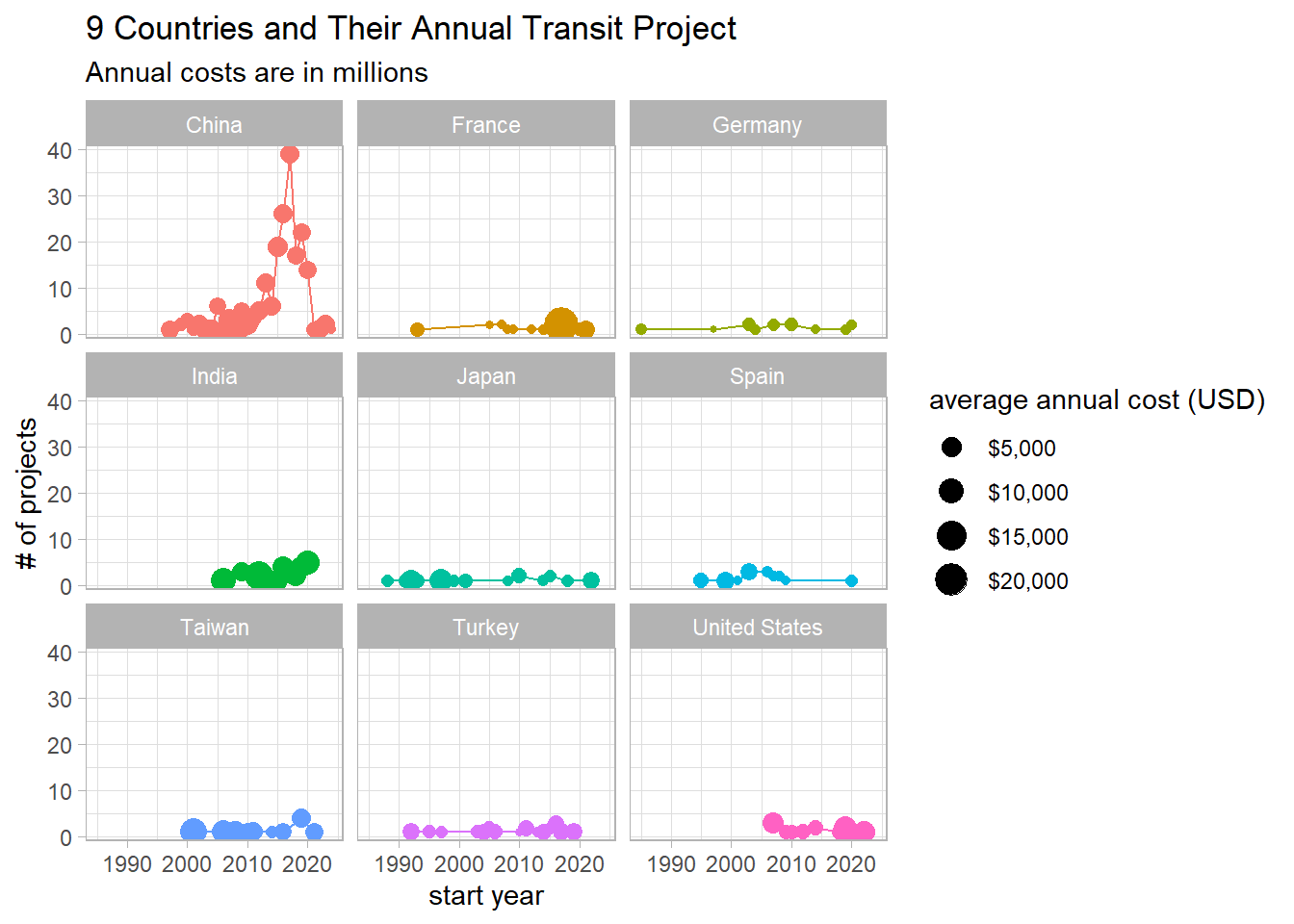
The relationship between transit length and # of years to finish:
transit_cost %>%
  ggplot(aes(length, project_duration, color = country)) +
  geom_point(alpha = 0.7, aes(size = cost_km_usd)) +
  geom_smooth(method = "lm", aes(group = 1), se = F) +
  geom_text(aes(label = country), check_overlap = T, vjust = 1, hjust = 1) +
  scale_color_discrete(guide = "none") +
  scale_x_log10() +
  scale_size_continuous(label = dollar) +
  labs(x = "length (km)",
       y = "# of years to finish",
size = "cost per km (USD in millions)") 
The length of the project does not necessarily indicate how long it takes to finish.
p1 <- transit_cost %>%
  group_by(start_year) %>%
  slice_max(cost_usd, n = 1) %>%
  ungroup() %>%
  ggplot(aes(start_year, cost_usd, fill = country_name)) +
  geom_col(show.legend = F) +
  geom_text(aes(label = country_name), check_overlap = T, vjust = 0, hjust = 0.5, size = 3) +
  scale_x_continuous(breaks = seq(1980, 2025, 5)) +
  scale_y_continuous(labels = dollar) +
  labs(x = "start year",
       y = "total cost (USD in millions)",
       title = "The Most Expensive Project Per Year",
       subtitle = "Being evaluated by the total cost")


p2 <- transit_cost %>%
  group_by(start_year) %>%
  slice_max(cost_km_usd, n = 1) %>%
  ungroup() %>%
  ggplot(aes(start_year, cost_km_usd, fill = country_name)) +
  geom_col(show.legend = F) +
  geom_text(aes(label = country_name), check_overlap = T, vjust = 0, hjust = 0.5, size = 3) +
  scale_x_continuous(breaks = seq(1980, 2025, 5)) +
  scale_y_continuous(labels = dollar) +
  labs(x = "start year",
       y = "average cost (USD in millions)",
       title = "The Most Expensive Project Per Year",
       subtitle = "Being evaluated by the average cost")

p1/p2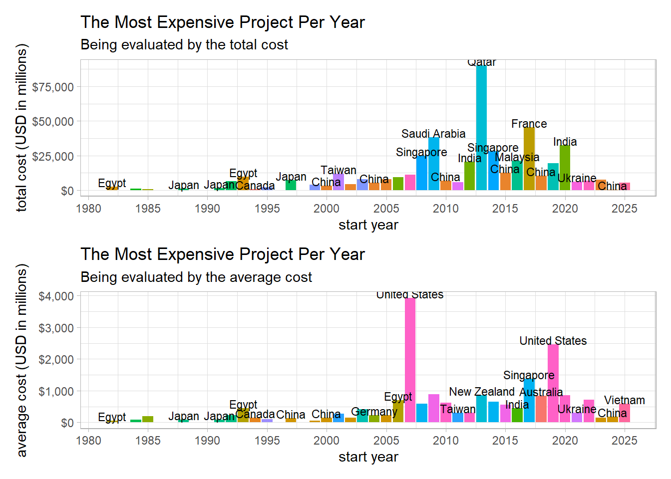
transit_cost %>%
  group_by(country, start_year) %>%
  summarize(avg_cost = mean(cost_km_usd, na.rm = T)) %>%
  ungroup() %>%
  arrange(desc(avg_cost)) %>%
  group_by(start_year) %>%
  slice_max(avg_cost, n = 1) %>%
  ungroup() %>%
  filter(!is.na(start_year)) %>%
  mutate(country_year = paste0(country, "(", start_year, ")"),
         country_year = fct_reorder(country_year, parse_number(country_year))) %>%
  ggplot(aes(avg_cost, country_year, fill = avg_cost)) +
  geom_col(show.legend = F) +
  labs(x = "average cost per km (USD in millions)",
       y = "country and year",
       title = "The Most Annual Expensive Transit Project",
       subtitle = "The cost is evaluated by USD in millions per km")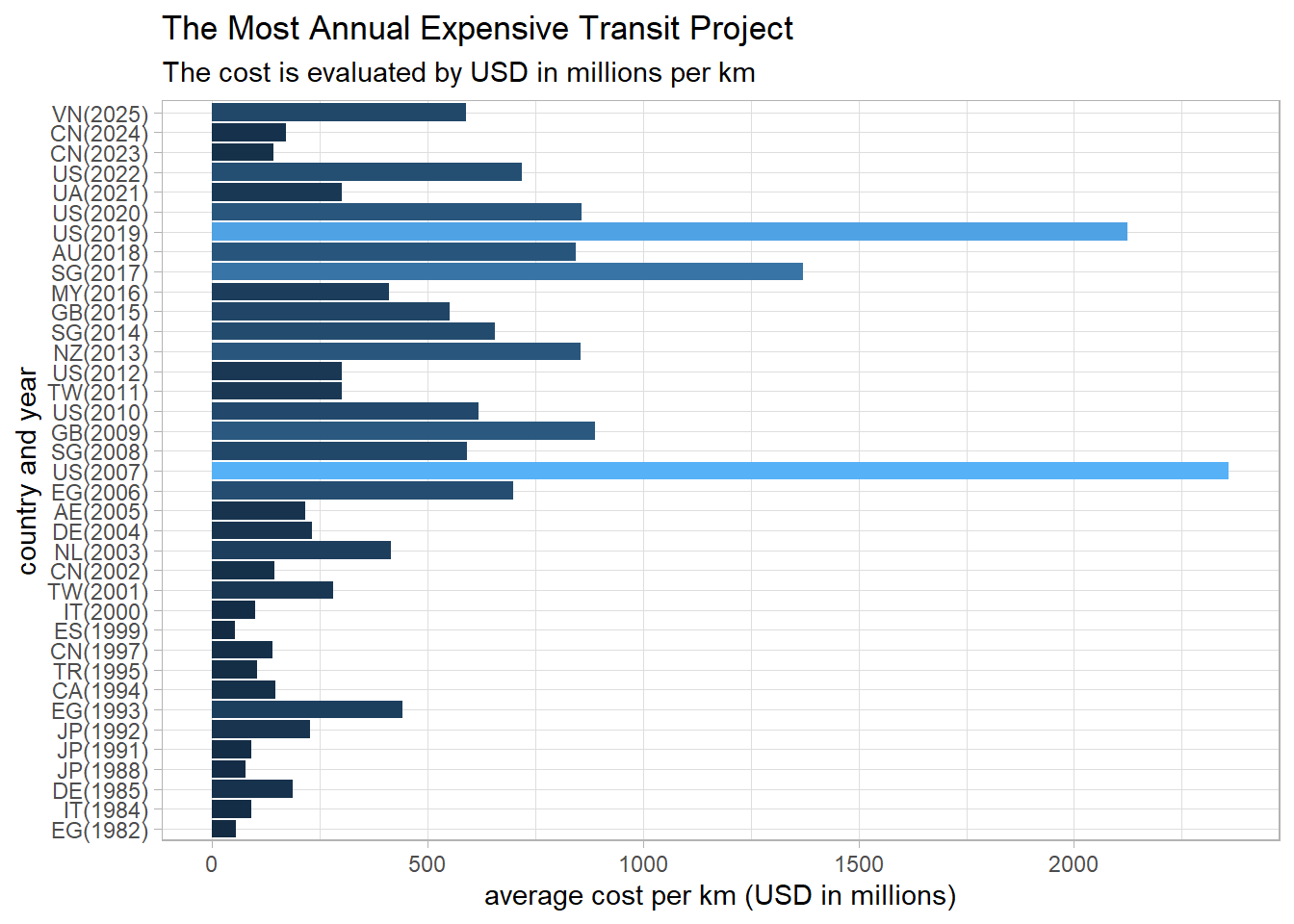
How much can each country build in a year (km)?
transit_cost %>%
  filter(tunnel_per == "100.00%") %>%
  mutate(efficiency = length/project_duration) %>%
  group_by(country_name) %>%
  summarize(avg_km = mean(efficiency, na.rm = T),
            n = n()) %>%
  filter(n > 5) %>%
  ungroup() %>%
  mutate(country_name = fct_reorder(country_name, avg_km)) %>%
  ggplot(aes(avg_km, country_name)) +
  geom_col() +
  labs(x = "average KM being constructed per year",
       y = "",
title = "The Efficiency for Building Transit System per Country") 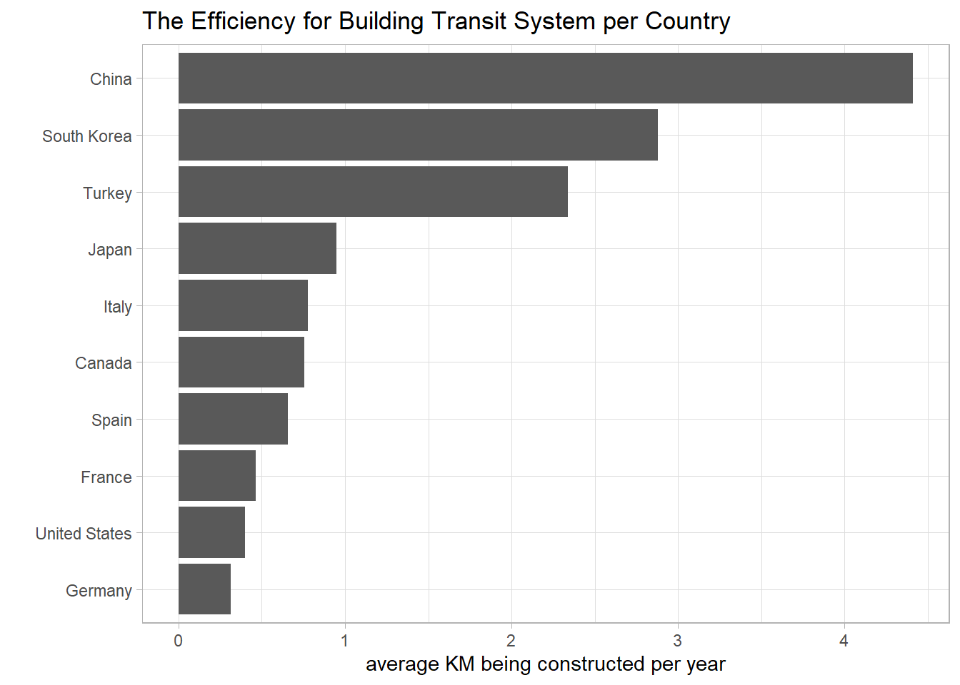
China is the most efficient country and it can build more than 4 KMs per year on average.