Analyzing Art Collections

In this blog post, I will analyze data about art collections and the respective artists. The two datasets come from TidyTuesday. If we have more than one dataset, naturally it would be a natural idea to join them together, if it is able to do so.

library(tidyverse)
library(tidytext)
library(tidylo)
theme_set(theme_bw())

artwork <- read_csv('https://raw.githubusercontent.com/rfordatascience/tidytuesday/master/data/2021/2021-01-12/artwork.csv')

artists <- read_csv("https://github.com/tategallery/collection/raw/master/artist_data.csv")

Join artwork and artists together:

art_joined <- artwork %>%
  select(artist, title, dateText, medium, creditLine, year, acquisitionYear, width, height, depth, units) %>%
  left_join(artists %>% select(-id, -url), by = c("artist" = "name")) %>%
  separate(artist, into = c("family_name", "first_name"), sep = ",\\s") %>%
  janitor::clean_names() %>%
  mutate(name = paste(first_name, family_name),
         name = str_remove_all(name, "NA |\\(\\?\\)\\s"),
         age = year_of_death - year_of_birth + 1,
         area_m_square = width * height / 100000,
         decade = 10 * (year %/% 10)) 

art_joined

## # A tibble: 69,319 x 22
##    family_name first_name title               date_text medium credit_line  year
##    <chr>       <chr>      <chr>               <chr>     <chr>  <chr>       <dbl>
##  1 Blake       Robert     A Figure Bowing be~ date not~ Water~ Presented ~    NA
##  2 Blake       Robert     Two Drawings of Fr~ date not~ Graph~ Presented ~    NA
##  3 Blake       Robert     The Preaching of W~ ?c.1785   Graph~ Presented ~  1785
##  4 Blake       Robert     Six Drawings of Fi~ date not~ Graph~ Presented ~    NA
##  5 Blake       William    The Circle of the ~ 1826–7, ~ Line ~ Purchased ~  1826
##  6 Blake       William    Ciampolo the Barra~ 1826–7, ~ Line ~ Purchased ~  1826
##  7 Blake       William    The Baffled Devils~ 1826–7, ~ Line ~ Purchased ~  1826
##  8 Blake       William    The Six-Footed Ser~ 1826–7, ~ Line ~ Purchased ~  1826
##  9 Blake       William    The Serpent Attack~ 1826–7, ~ Line ~ Purchased ~  1826
## 10 Blake       William    The Pit of Disease~ 1826–7, ~ Line ~ Purchased ~  1826
## # ... with 69,309 more rows, and 15 more variables: acquisition_year <dbl>,
## #   width <dbl>, height <dbl>, depth <dbl>, units <chr>, gender <chr>,
## #   dates <chr>, year_of_birth <dbl>, year_of_death <dbl>,
## #   place_of_birth <chr>, place_of_death <chr>, name <chr>, age <dbl>,
## #   area_m_square <dbl>, decade <dbl>

The most popular medium:

art_joined %>%
  filter(!is.na(medium),
         !is.na(decade)) %>%
  count(decade, medium, sort = T) %>%
  filter(n > 50) %>%
  group_by(decade) %>%
  slice_max(n, n = 1) %>%
  ungroup() %>%
  ggplot(aes(decade, n, fill = medium)) +
  geom_col() +
  scale_y_log10() +
  scale_x_continuous(breaks = seq(1700, 2000, 50)) +
  labs(y = "# of artwork",
       title = "The Most Popular Medium per Decade")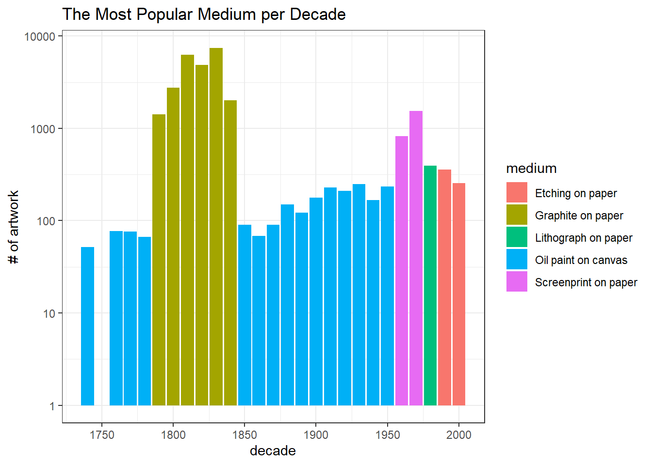

When did the artwork come along?

art_joined %>%
  count(year) %>%
  filter(!is.na(year)) %>%
  ggplot(aes(year, n)) +
  geom_line() +
  scale_x_continuous(breaks = seq(1600, 2000, 50)) +
  labs(y = "# of artwork",
       title = "Yearly # of Artwork Count")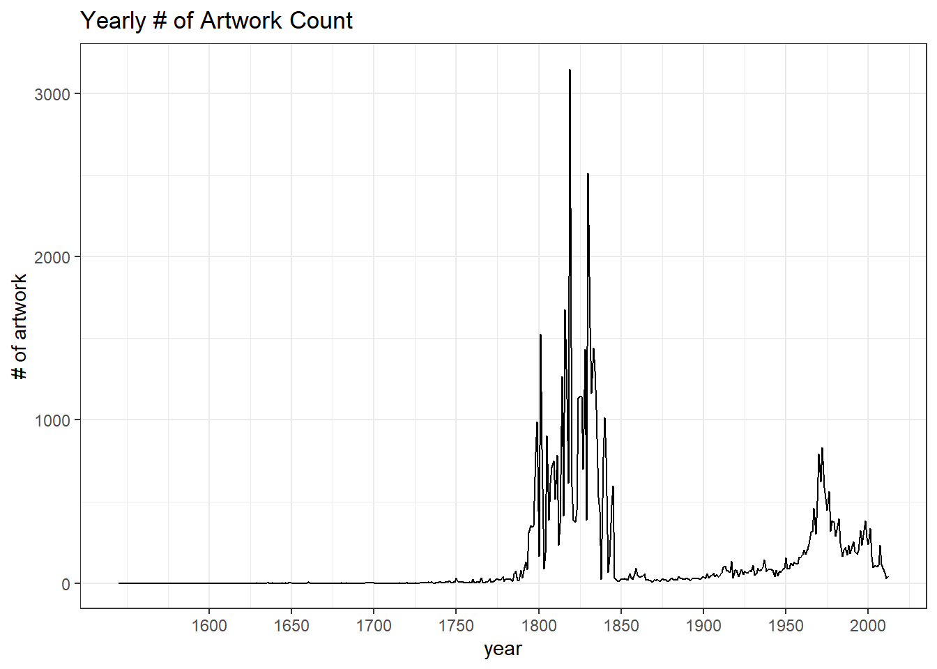 

A significant number of pieces of art are from early 1800 to 1850.

art_joined %>%
  filter(!str_detect(title, "\\["),
         !title %in% c("Blank", "Untitled"),
         !str_detect(title, ", Etc\\."),
         str_length(title) < 30) %>%
  count(title, decade, sort = T) %>%
  filter(n > 20) %>%
  bind_log_odds(decade, title, n) %>%
  filter(log_odds_weighted != Inf) %>%
  group_by(title) %>%
  slice_max(log_odds_weighted, n = 1) %>%
  ungroup() %>%
  mutate(title = paste0(title, "(", decade, ")")) %>%
  mutate(title = fct_reorder(title, log_odds_weighted)) %>%
  ggplot(aes(log_odds_weighted, title, fill = n)) +
  geom_col() +
  labs(x = "weigthed log odds",
       y = "title and year",
       fill = "# of artwork",
       title = "What Title is Most Characteristic to Decade?")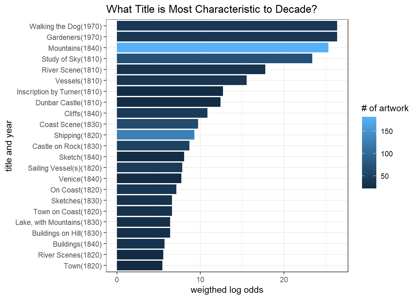

Who spent most time on one artwork piece on average?

art_joined %>%
  add_count(name, age) %>%
  distinct(name, age, n) %>%
  filter(n > 50,
         age < 100) %>%
  mutate(avg_yr_per_work = age/n) %>%
  arrange(desc(avg_yr_per_work)) %>%
  head(10) %>%
  mutate(name = paste0(name, "(", age, ")"),
         name = fct_reorder(name, avg_yr_per_work)) %>%
  ggplot(aes(avg_yr_per_work, name, fill = n)) +
  geom_col() +
  labs(x = "average years per artwork",
       y = "name and age",
       fill = "# of artwork pieces",
       title = "Top 10 Artists Spending Longest Time on Artwork")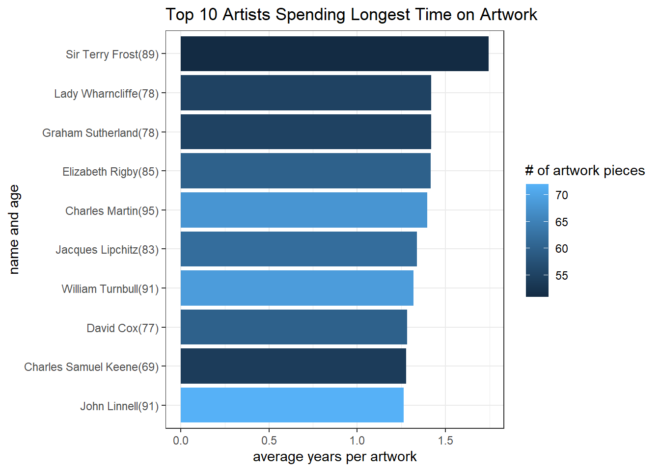

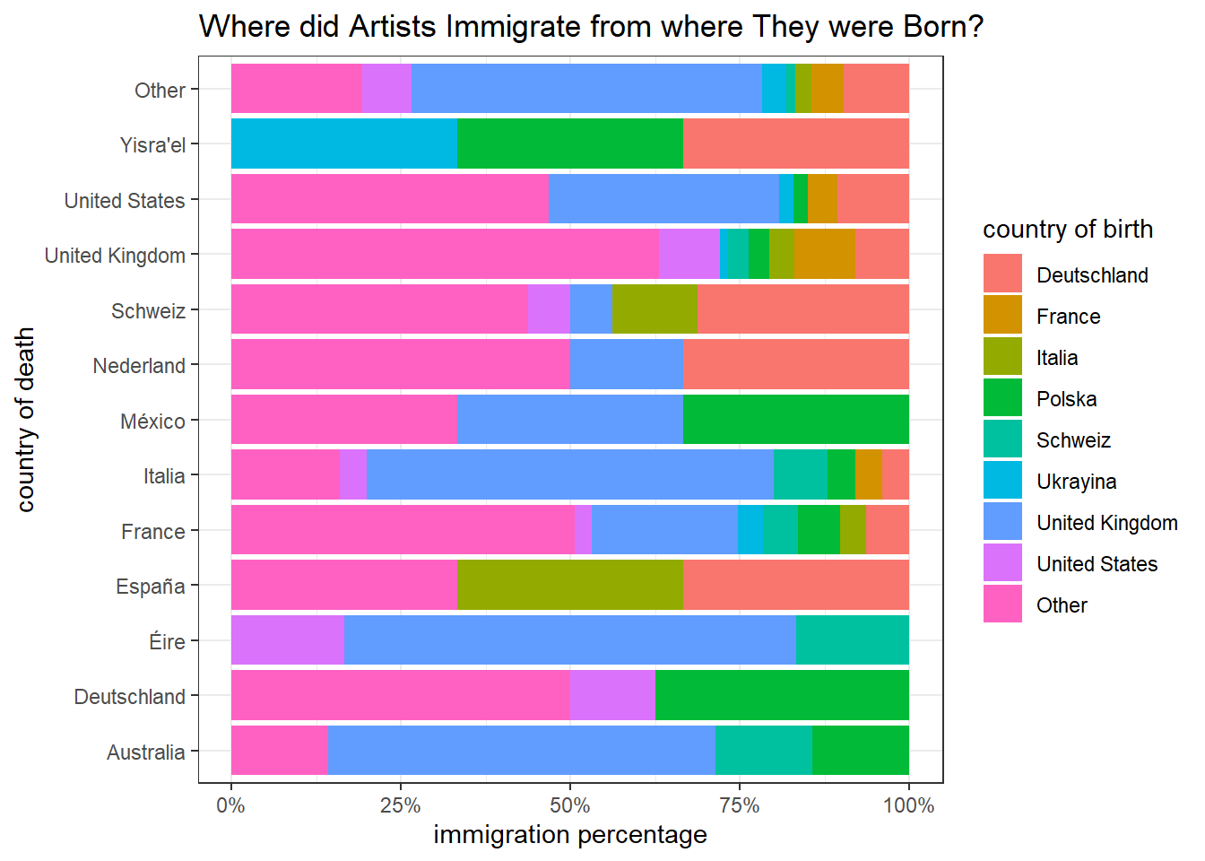
art_joined %>%
  mutate(birth_country = str_remove(place_of_birth, "^.+,\\s"),
         death_country = str_remove(place_of_death, "^.+,\\s"),
         immigration = if_else(birth_country == death_country, "Same", "Immigration")) %>%
  distinct(name, birth_country, .keep_all = T) %>%
  filter(immigration == "Immigration") %>%
  count(birth_country, death_country, sort = T) %>% 
  mutate(birth_country = fct_lump(birth_country, n = 5),
         death_country = fct_lump(death_country, n = 10)) %>%
  group_by(death_country) %>%
  mutate(pct_death = n/sum(n)) %>%
  ungroup() %>%
  ggplot(aes(pct_death, death_country, fill = birth_country)) +
  geom_col() +
  scale_x_continuous(labels = scales::percent) +
  labs(x = "immigration percentage",
       y = "country of death",
       fill = "country of birth",
       title = "Where did Artists Immigrate from where They were Born?")