HBCU Enrollment Data Visualization
In this blog post, I will analyze the data about HBCU enrollment from TidyTuesday. Personally, I don’t know what HBCU stands for prior to analyzing the data, and hopefully I can use data visualization to understand it better.
Load the packages and set up the theme for plots:
library(tidyverse)
library(janitor)
library(patchwork)
theme_set(theme_bw())
Load and clean up the data:
hbcu_all <- read_csv("https://raw.githubusercontent.com/rfordatascience/tidytuesday/master/data/2021/2021-02-02/hbcu_all.csv") %>%
  clean_names()

hs_students <- read_csv("https://raw.githubusercontent.com/rfordatascience/tidytuesday/master/data/2021/2021-02-02/hs_students.csv") %>%
  clean_names() %>%
  mutate(total = fct_recode(as.character(total),
                            "1910" = "19103",
                            "1920" = "19203",
                            "1930" = "19303"))

hbcu_black <- read_csv("https://raw.githubusercontent.com/rfordatascience/tidytuesday/master/data/2021/2021-02-02/hbcu_black.csv") %>%
  clean_names()

hbcu_all
## # A tibble: 32 x 12
## year total_enrollment males females x4_year x2_year total_public
## <dbl> <dbl> <dbl> <dbl> <dbl> <dbl> <dbl>
## 1 1976 222613 104669 117944 206676 15937 156836
## 2 1980 233557 106387 127170 218009 15548 168217
## 3 1982 228371 104897 123474 212017 16354 165871
## 4 1984 227519 102823 124696 212844 14675 164116
## 5 1986 223275 97523 125752 207231 16044 162048
## 6 1988 239755 100561 139194 223250 16505 173672
## 7 1990 257152 105157 151995 240497 16655 187046
## 8 1991 269335 110442 158893 252093 17242 197847
## 9 1992 279541 114622 164919 261089 18452 204966
## 10 1993 282856 116397 166459 262430 20426 208197
## # ... with 22 more rows, and 5 more variables: x4_year_public <dbl>,
## # x2_year_public <dbl>, total_private <dbl>, x4_year_private <dbl>,
## # x2_year_private <dbl>Data processing:
column_name_change <- . %>%
  rename(`Total Enrollment` = total_enrollment,
         Male = males,
         Female = females,
         `Year 4` = x4_year,
         `Year 2` = x2_year,
         `Total Public` = total_public,
         `Total Private` = total_private,
         `Public Year 4` = x4_year_public,
         `Public Year 2` = x2_year_public,
         `Private Year 4` = x4_year_private,
         `Private Year 2` = x2_year_private) %>%
  pivot_longer(2:12,
               names_to = "student",
               values_to = "count")


hbcu_all_long <- hbcu_all %>%
  column_name_change

hbcu_all_long
## # A tibble: 352 x 3
## year student count
## <dbl> <chr> <dbl>
## 1 1976 Total Enrollment 222613
## 2 1976 Male 104669
## 3 1976 Female 117944
## 4 1976 Year 4 206676
## 5 1976 Year 2 15937
## 6 1976 Total Public 156836
## 7 1976 Public Year 4 143528
## 8 1976 Public Year 2 13308
## 9 1976 Total Private 65777
## 10 1976 Private Year 4 63148
## # ... with 342 more rowsNow let’s visualize HBCU enrollemnt across various sectors. Here functional programming is used, map() and reduce() in particular.
hbcu_line_scatter <- function(vec, tbl) {

  tbl %>%
  filter(student %in% vec) %>%
  mutate(student = fct_reorder(student, -count, sum)) %>%
  ggplot(aes(year, count, color = student)) +
  geom_line() +
  geom_point() +
  labs(color = NULL,
       x = NULL,
       y = "# of enrollment",
       title = "Yearly # of HBCU Enrollment") +
  theme(legend.position = "bottom")
}

hbcu_plots <- function(hbcu_tbl = hbcu_all_long) {

  plots <- map(list(c("Male", "Female"),
           c("Year 4", "Year 2"),
           c("Total Public", "Total Private")),
      hbcu_line_scatter,
      tbl = hbcu_tbl)

  return(plots)
}
reduce(hbcu_plots(), `/`)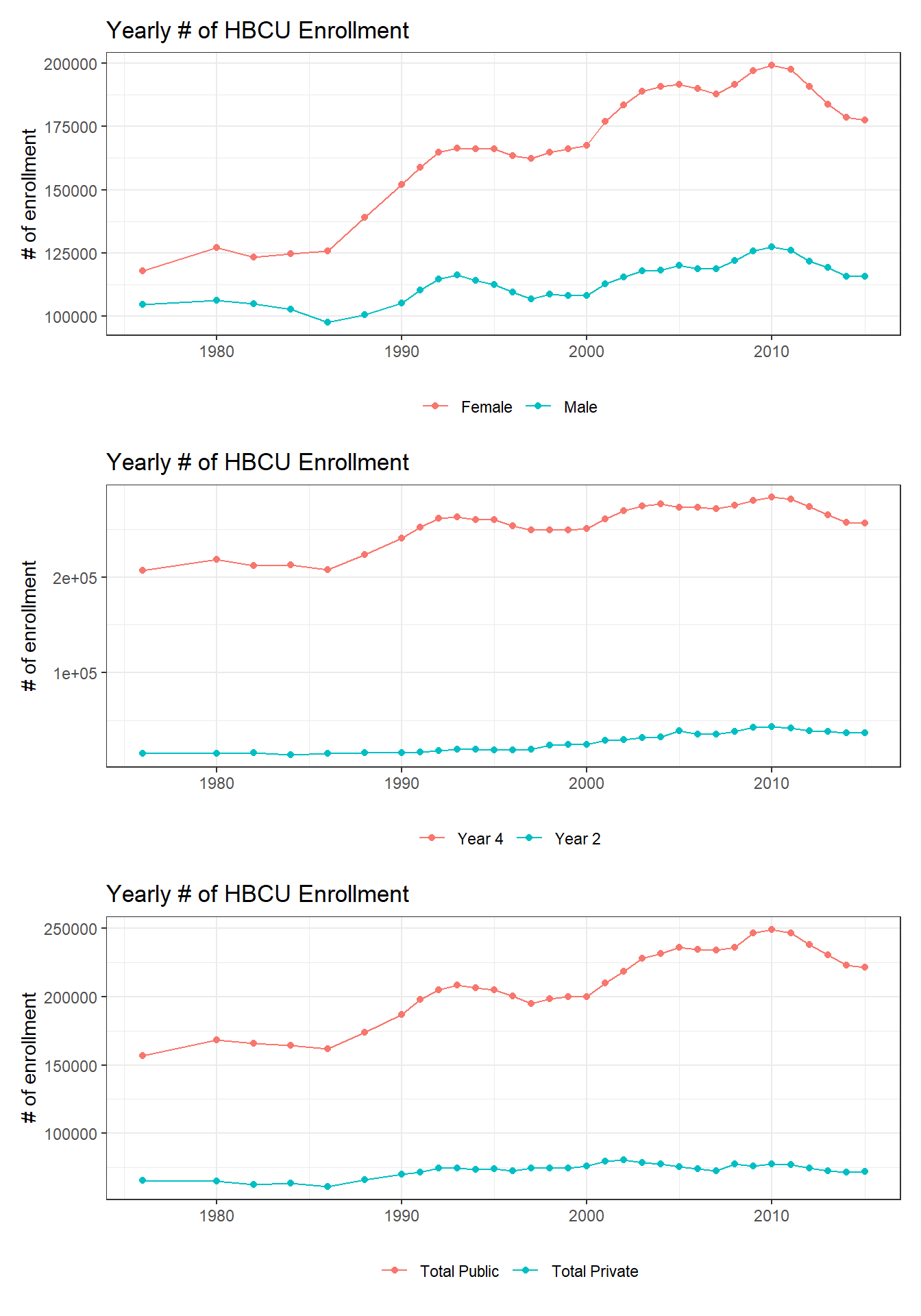
There are much more female students than male over the years, and by no means can the number of private students be comparable to its public counterpart. Also, the majority of enrollment are 4-year college students.
We can use the same structure set up above on hbcu_black:
reduce(hbcu_plots(hbcu_black %>% column_name_change),
       `/`)
We actually observed the very similar, if not the same, trend for the black student enrollment as the overall enrollment.
hs_long <- hs_students %>%
  mutate(across(is.numeric, as.character)) %>%
  pivot_longer(cols = c(2:19),
               names_to = "race",
               values_to = "pct") %>%
  filter(str_detect(pct, "[:digit:]")) %>%
  mutate(pct = as.numeric(pct),
         race = str_remove(race, "1$")) %>%
  rename(year = total)

hs_long
## # A tibble: 451 x 3
## year race pct
## <fct> <chr> <dbl>
## 1 1910 total_percent_of_all_persons_age_25_and_over 13.5
## 2 1920 total_percent_of_all_persons_age_25_and_over 16.4
## 3 1930 total_percent_of_all_persons_age_25_and_over 19.1
## 4 1940 total_percent_of_all_persons_age_25_and_over 24.5
## 5 1940 white 26.1
## 6 1940 black 7.7
## 7 1950 total_percent_of_all_persons_age_25_and_over 34.3
## 8 1950 white 36.4
## 9 1950 black 13.7
## 10 1960 total_percent_of_all_persons_age_25_and_over 41.1
## # ... with 441 more rowshs_long %>%
filter(race == "total_percent_of_all_persons_age_25_and_over") %>%
ggplot(aes(year, pct, group = 1)) +
geom_line() +
geom_point() +
theme(axis.text.x = element_text(angle = 90)) +
scale_y_continuous(labels = scales::percent_format(scale = 1)) +
labs(x = NULL,
y = "percentage of age 25 and above",
title = "Yearly Percentage of All Persons Age 25 and Over") 
hs_long %>%
  mutate(year = as.numeric(as.character(year))) %>%
  filter(!str_detect(race, "standard"),
         str_detect(race, "white|black|total_asian|indian")) %>%
  mutate(race = str_to_title(fct_recode(race,
                                        "asian" = "total_asian_pacific_islander",
                                        "native indian" = "american_indian_alaska_native")),
         race = fct_reorder(race, -pct, last)) %>%
  ggplot(aes(year, pct, color = race, group = race)) +
  geom_line() +
  geom_point() +
  scale_y_continuous(labels = scales::percent_format(scale = 1)) +
  theme(axis.text.x = element_text(angle = 90)) +
  labs(x = "",
       y = "percentage of this race",
       color = "",
       title = "Percentage of Various Races graduating HS")
When evaluating the plot, we can see that in 1940 only black and white students being recorded graduating from HS, and Asian students began to emerge at the end of 1980s, followed by the Native Indian students.