Super Bowl Ads Data Visualization & Modeling
This blog post analyzes the ads for the Super Bowl. This is an intersting dataset coming from TidyTuesday. In this post, I will visualize the data from various perspectives, and use machine learning model to analyze it with the tidymodels meta-package used.
Load the packages:
library(tidyverse)
library(tidylo)
library(tidytext)
library(tidymodels)
library(broom)
theme_set(theme_bw())
Load the dataset with some simple cleaning:
youtube <- read_csv('https://raw.githubusercontent.com/rfordatascience/tidytuesday/master/data/2021/2021-03-02/youtube.csv') %>%
  select(-contains("url"), -etag, -kind, -thumbnail)

youtube
## # A tibble: 247 x 20
## year brand funny show_product_qu~ patriotic celebrity danger animals use_sex
## <dbl> <chr> <lgl> <lgl> <lgl> <lgl> <lgl> <lgl> <lgl>
## 1 2018 Toyo~ FALSE FALSE FALSE FALSE FALSE FALSE FALSE
## 2 2020 Bud ~ TRUE TRUE FALSE TRUE TRUE FALSE FALSE
## 3 2006 Bud ~ TRUE FALSE FALSE FALSE TRUE TRUE FALSE
## 4 2018 Hynu~ FALSE TRUE FALSE FALSE FALSE FALSE FALSE
## 5 2003 Bud ~ TRUE TRUE FALSE FALSE TRUE TRUE TRUE
## 6 2020 Toyo~ TRUE TRUE FALSE TRUE TRUE TRUE FALSE
## 7 2020 Coca~ TRUE FALSE FALSE TRUE FALSE TRUE FALSE
## 8 2020 Kia FALSE FALSE FALSE TRUE FALSE FALSE FALSE
## 9 2020 Hynu~ TRUE TRUE FALSE TRUE FALSE TRUE FALSE
## 10 2020 Budw~ FALSE TRUE TRUE TRUE TRUE FALSE FALSE
## # ... with 237 more rows, and 11 more variables: id <chr>, view_count <dbl>,
## # like_count <dbl>, dislike_count <dbl>, favorite_count <dbl>,
## # comment_count <dbl>, published_at <dttm>, title <chr>, description <chr>,
## # channel_title <chr>, category_id <dbl>Ads category:
youtube_long <- youtube %>%
  pivot_longer(funny:use_sex, names_to = "kind", values_to = "if_contain") %>%
  mutate(kind = str_replace_all(kind, "_", " "))

youtube_long %>%
  count(year, kind, sort = T) %>%
  mutate(kind = fct_reorder(kind, n, sum)) %>%
  ggplot(aes(year, n, color = kind)) +
  geom_point() +
  geom_line() +
  scale_y_continuous(breaks = seq(1,12)) +
  facet_wrap(~kind) +
  theme(legend.position = "none") +
  labs(y = "# of ads",
       title = "Yearly # of Ads per Category")
youtube_long %>%
  filter(if_contain) %>%
  mutate(kind = fct_reorder(kind, view_count, na.rm = T)) %>%
  ggplot(aes(view_count, kind, fill = kind)) +
  geom_boxplot(show.legend = F) +
  scale_x_log10() +
  labs(x = "# of views",
       y = "",
       title = "# of Views per Category")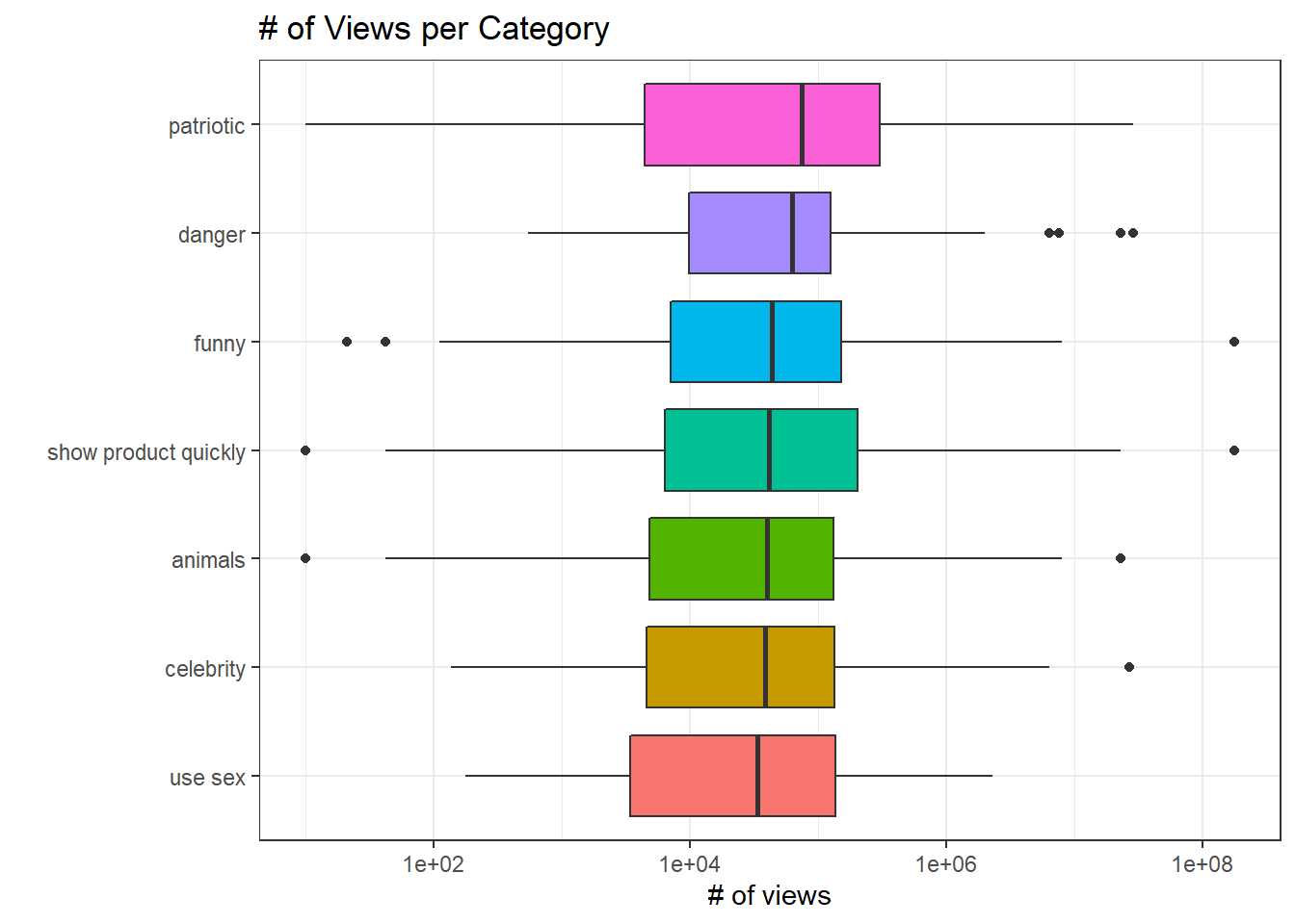
patriotic is the most popular category among the ads, and use sex is the least one. One thing worth mention is there are a few most watched ads from the funny and show product quickly categories.
youtube %>%
  mutate(brand_year = paste0(brand, "(", year, ")")) %>%
  ggplot(aes(view_count, like_count, color = factor(year))) +
  geom_point() +
  geom_text(aes(label = brand_year),
            vjust = 1,
            hjust = 1,
            check_overlap = T) +
  scale_x_log10() +
  scale_y_log10() +
  theme(legend.position = "none") +
  labs(x = "# of views",
       y = "# of likes",
title = "# of Views and # of Likes") 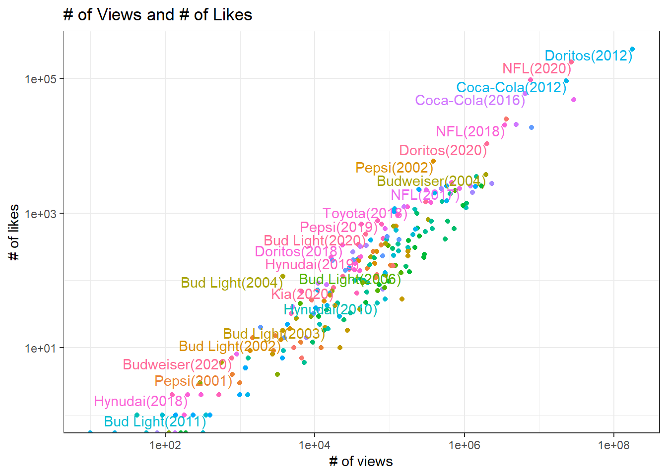
There is a positive and linear relationship between them, meaning more views, more likes.
youtube %>%
  mutate(brand = fct_reorder(brand, view_count, na.rm = T)) %>%
  ggplot(aes(view_count, brand)) +
  geom_boxplot() +
  scale_x_log10() +
  labs(x = "# of views",
       y = NULL,
title = "Brands and Their Views") 
NFL has the most watched ads in general, and Hynudai the least.
youtube_long %>%
  filter(if_contain) %>%
  count(brand, kind) %>%
  bind_log_odds(brand, kind, n) %>%
  mutate(brand = fct_reorder(brand, log_odds_weighted, sum)) %>%
  ggplot(aes(log_odds_weighted, brand, fill = kind)) +
  geom_col(position = "dodge") +
  labs(x = "weighted log odds",
       y = NULL,
       fill = NULL,
       title = "Weighted Log Odds for All Brands per Category")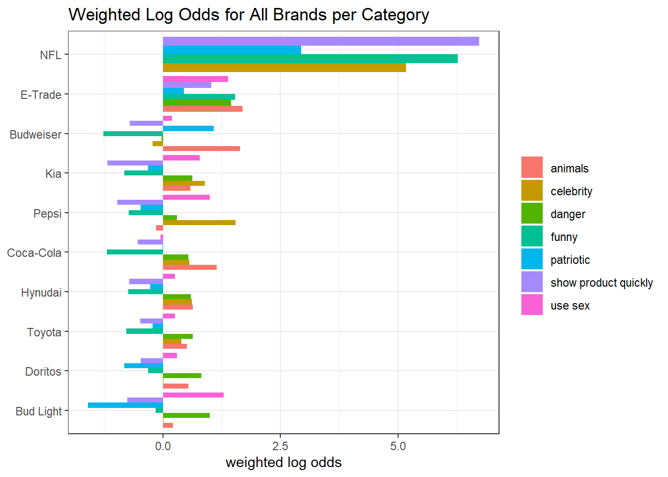
The NFL ads are the most patriotic, while ads of Bud Light and E-Trade weight more on using sex than other brands.
Modeling:
linear_reg() %>%
  fit(view_count ~ year + brand + funny + show_product_quickly + patriotic +
                         celebrity + danger + animals + use_sex, data = youtube) %>%
  tidy() %>%
  mutate(term = str_remove_all(term, "brand|TRUE"),
         term = str_replace_all(term, "_", " ")) %>%
  filter(term != "(Intercept)") %>%
  mutate(term = fct_reorder(term, estimate)) %>%
  ggplot(aes(estimate, term, color = p.value < 0.05)) +
  geom_point() +
  geom_errorbarh(aes(xmin = estimate - std.error,
                     xmax = estimate + std.error),
                 height = 0.2) +
  geom_vline(xintercept = 0, lty = 2) +
  labs(y = NULL,
       title = "Linear Regression Estimates for Predictors",
       subtitle = "View count is the response variable")
youtube_long %>%
  select(year, kind, if_contain) %>%
  group_by(kind) %>%
  summarize(model = list(glm(if_contain ~ year, family = "binomial"))) %>%
  ungroup() %>%
  mutate(tidied = map(model, tidy)) %>%
  unnest(tidied) %>%
  filter(term != "(Intercept)") %>%
  mutate(kind = fct_reorder(kind, estimate)) %>%
  ggplot(aes(estimate, kind)) +
  geom_point(aes(color = p.value < 0.05)) +
  geom_errorbarh(aes(xmin = estimate - std.error,
                     xmax = estimate + std.error),
                 height = 0.2) +
  geom_vline(xintercept = 0, lty = 2) +
  labs(y = NULL,
       title = "Logistic Regreesion Estimate",
       subtitle = "The model is categroy ~ year")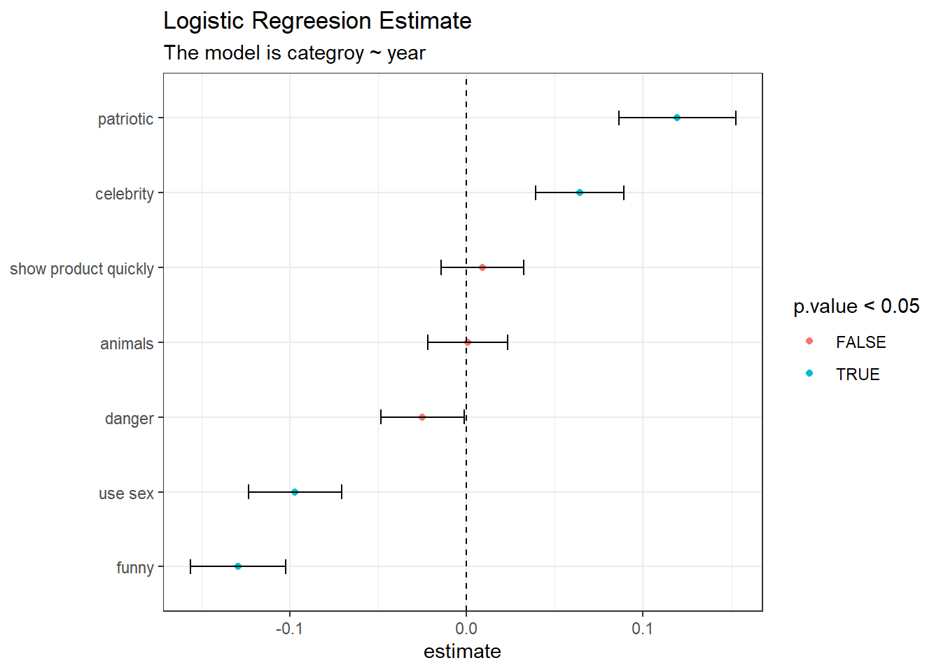
As the year increases, the ads tend to be more patriotic and more celebrity presented. At the same time, it is less funny and using less sex.
Description words:
youtube %>%
  unnest_tokens(word, description) %>%
  anti_join(stop_words) %>%
  select(brand, word) %>%
  count(brand, word) %>%
  bind_log_odds(brand, word, n) %>%
  group_by(brand) %>%
  slice_max(log_odds_weighted, n = 5) %>%
  ungroup() %>%
  mutate(word = reorder_within(word, log_odds_weighted, brand)) %>%
  ggplot(aes(log_odds_weighted, word, fill = brand)) +
  geom_col(show.legend = F) +
  scale_y_reordered() +
  facet_wrap(~brand, scales = "free_y", ncol = 5) +
  theme(strip.text = element_text(size = 12)) +
  labs(x = "weighted log odds",
       y = "description word",
       title = "Top 5 Words with the Largest Weighted Log Odds per Brand")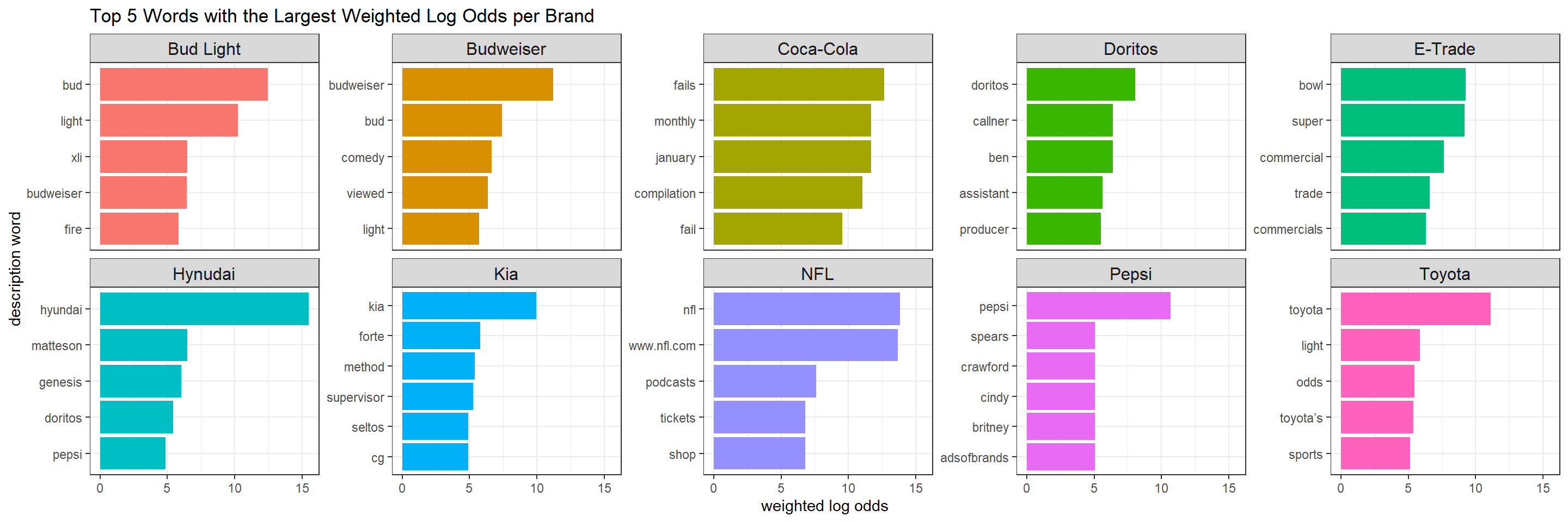
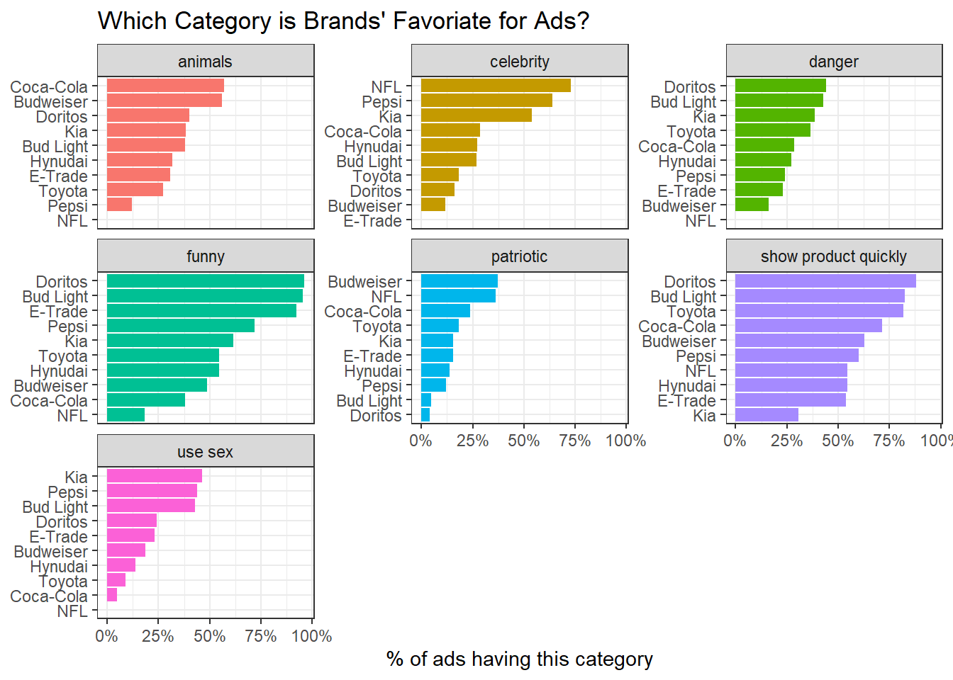
Ad category usage for brands:
youtube_long %>%
  group_by(brand, kind) %>%
  summarize(avg_kind = mean(if_contain)) %>%
  ungroup() %>%
  mutate(brand = reorder_within(brand, avg_kind, kind)) %>%
  ggplot(aes(avg_kind, brand, fill = kind)) +
  geom_col() +
  scale_y_reordered() +
  facet_wrap(~kind, scales = "free_y") +
  theme(legend.position = "none") +
  scale_x_continuous(labels = percent) +
  labs(x = "% of ads having this category",
       y = NULL,
       title = "Which Category is Brands' Favoriate for Ads?")