Bechdel Test Data Visualization (with tidymodels LASSO used)
This blog post analyzes the Bechdel test dataset from TidyTuesday for a wide range of movies.
library(tidyverse)
library(lubridate)
library(scales)
library(tidytext)
library(glmnet)
library(Matrix)
library(tidymodels)
library(vip)
theme_set(theme_bw())
raw_bechdel <- read_csv('https://raw.githubusercontent.com/rfordatascience/tidytuesday/master/data/2021/2021-03-09/raw_bechdel.csv') %>%
rename(imdb = imdb_id) %>%
mutate(decade = 10 * (year %/%10))
movies <- read_csv('https://raw.githubusercontent.com/rfordatascience/tidytuesday/master/data/2021/2021-03-09/movies.csv') %>%
mutate(imdb = str_remove(imdb, "tt"))Decade-wise bechdel ratings:
raw_bechdel %>%
  group_by(decade) %>%
  summarize(`mean rating` = mean(rating),
            `median rating` = median(rating),
            n = n()) %>%
  ungroup() %>%
  pivot_longer(cols = 2:3, names_to = "metric")  %>%
  mutate(metric = fct_reorder(metric, -value, sum)) %>%
  ggplot(aes(decade, value, color = metric)) +
  geom_line(size = 1) +
  geom_point(aes(size = n)) +
  labs(y = "bechdel rating",
       color = NULL,
       size = "# of movies",
       title = "Bechdel Movie Ratings per Decade (Mean & Median)")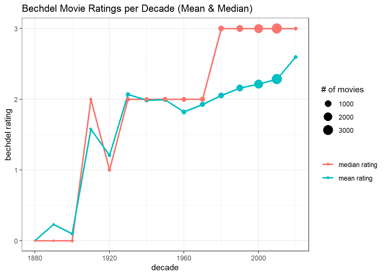
Clearly, there is an improvement on bechdel ratings decade after decade with some dropping in the 1920s.
Join both datasets together:
movies %>%
  anti_join(raw_bechdel, by = c("imdb"))
## # A tibble: 1 x 34
## year imdb title test clean_test binary budget domgross intgross code
## <dbl> <chr> <chr> <chr> <chr> <chr> <dbl> <chr> <chr> <chr>
## 1 2012 1598828 One for ~ ok ok PASS 4.2e7 26414527 36197221 2012~
## # ... with 24 more variables: budget_2013 <dbl>, domgross_2013 <chr>,
## # intgross_2013 <chr>, period_code <dbl>, decade_code <dbl>, imdb_id <chr>,
## # plot <chr>, rated <chr>, response <lgl>, language <chr>, country <chr>,
## # writer <chr>, metascore <dbl>, imdb_rating <dbl>, director <chr>,
## # released <chr>, actors <chr>, genre <chr>, awards <chr>, runtime <chr>,
## # type <chr>, poster <chr>, imdb_votes <dbl>, error <lgl>It seems like there is only one movie that is in the movies tibble that isn’t present in the raw_bechdel one.
We just left join them:
movie_joined <- movies %>%
  left_join(raw_bechdel %>%
              transmute(imdb, bechdel_rating = rating), by = "imdb") %>%
  mutate(runtime = as.numeric(str_remove(runtime, " min"))) %>%
  select(-domgross, -intgross, -poster) %>%
  mutate(released = dmy(released)) %>%
  filter(!is.na(bechdel_rating))

movie_joined
## # A tibble: 1,793 x 32
## year imdb title test clean_test binary budget code budget_2013
## <dbl> <chr> <chr> <chr> <chr> <chr> <dbl> <chr> <dbl>
## 1 2013 1711425 21 & Over nota~ notalk FAIL 1.3 e7 2013~ 13000000
## 2 2012 1343727 Dredd 3D ok-d~ ok PASS 4.5 e7 2012~ 45658735
## 3 2013 2024544 12 Years a Sl~ nota~ notalk FAIL 2 e7 2013~ 20000000
## 4 2013 1272878 2 Guns nota~ notalk FAIL 6.1 e7 2013~ 61000000
## 5 2013 0453562 42 men men FAIL 4 e7 2013~ 40000000
## 6 2013 1335975 47 Ronin men men FAIL 2.25e8 2013~ 225000000
## 7 2013 1606378 A Good Day to~ nota~ notalk FAIL 9.2 e7 2013~ 92000000
## 8 2013 2194499 About Time ok-d~ ok PASS 1.2 e7 2013~ 12000000
## 9 2013 1814621 Admission ok ok PASS 1.3 e7 2013~ 13000000
## 10 2013 1815862 After Earth nota~ notalk FAIL 1.3 e8 2013~ 130000000
## # ... with 1,783 more rows, and 23 more variables: domgross_2013 <chr>,
## # intgross_2013 <chr>, period_code <dbl>, decade_code <dbl>, imdb_id <chr>,
## # plot <chr>, rated <chr>, response <lgl>, language <chr>, country <chr>,
## # writer <chr>, metascore <dbl>, imdb_rating <dbl>, director <chr>,
## # released <date>, actors <chr>, genre <chr>, awards <chr>, runtime <dbl>,
## # type <chr>, imdb_votes <dbl>, error <lgl>, bechdel_rating <dbl>movie_joined %>%
ggplot(aes(binary, runtime)) +
geom_boxplot() +
labs(x = "test result",
y = "movie runtime (minutes)",
title = "Movie Runtime and Bechdel Test")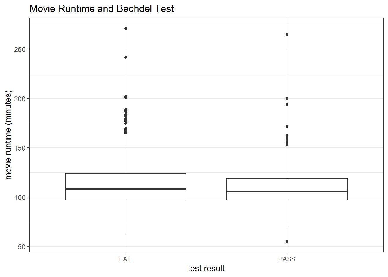
There doesn’t have a strong relationship between runtime and test results.
movie_joined %>%
  ggplot(aes(imdb_rating, bechdel_rating, color = binary)) +
  geom_jitter()
movie_joined %>%
  filter(!is.na(rated)) %>%
  count(rated, binary, sort = T) %>%
  add_count(rated, wt = n, name = "rated_total") %>%
  mutate(pct_rated_binary = n/rated_total,
         rated = fct_reorder(rated, pct_rated_binary, na.rm = T)) %>%
  ggplot(aes(binary, rated, fill = pct_rated_binary)) +
  geom_tile() +
  scale_fill_gradient(low = "red",
                      high = "green",
                      labels = percent) +
  labs(x = "pass bechdel test?",
       y = "",
       fill = "test result pct",
       title = "Movie Ratings and Bechdel Test Passing") +
  theme(panel.grid = element_blank())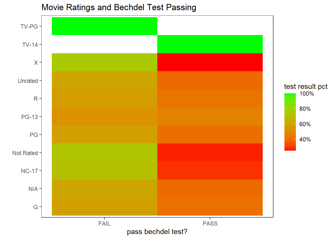
TV-PG failed on all bechdel testing, but TV-14 passed all.
movie_joined %>%
  mutate(profit_rate = (as.numeric(domgross_2013) + as.numeric(intgross_2013) - budget_2013)/budget_2013) %>%

  ggplot(aes(imdb_votes, profit_rate)) +
  geom_point(alpha = 0.6, aes(color = binary)) +
  geom_text(aes(label = title),
            vjust = 1,
            hjust = 1,
            check_overlap = T) +
  scale_x_log10() +
  scale_y_continuous(labels = percent) +
  labs(x = "IMDB votes",
       y = "profit rate",
       color = "test result",
       title = "Profit Rate and IMBD Votes",
       subtitle = "Profit includes both domestic and international")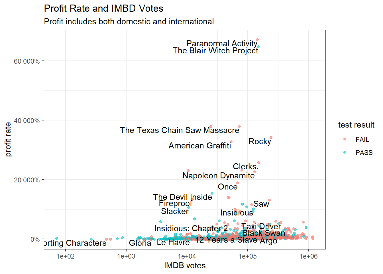
LASSO regression:
plot_matrix <- movie_joined %>%

  mutate(row_id = row_number()) %>%
  unnest_tokens(word, plot) %>%
  anti_join(stop_words) %>%
  add_count(word) %>%
  cast_sparse(row_id, word)

row_id <- as.integer(rownames(plot_matrix))
rating <- movie_joined$bechdel_rating[row_id]
cv_glmnet_model <- cv.glmnet(plot_matrix, rating)
plot(cv_glmnet_model)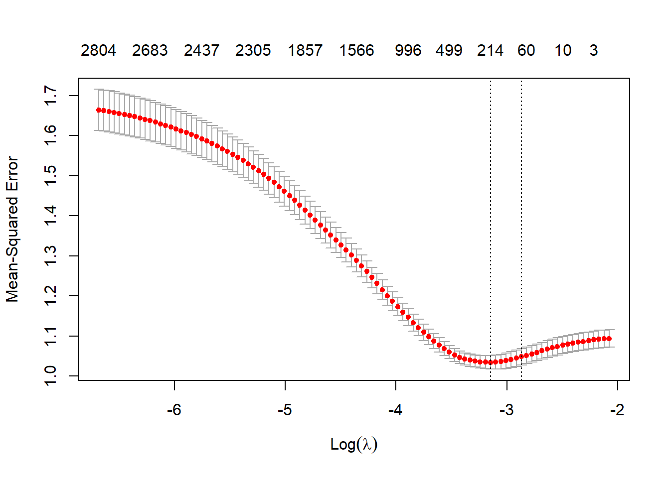
cv_glmnet_model$glmnet.fit %>%
  broom::tidy() %>%
  filter(!str_detect(term, "(Intercept)"),
         lambda == cv_glmnet_model$lambda.1se) %>%
  mutate(term = fct_reorder(term, estimate)) %>%
  ggplot(aes(estimate, term, fill = estimate > 0)) +
  geom_col() +
  theme(legend.position = "none") +
  labs(x = "lasso estimate",
       y = "",
       title = "LASSO Regression on Plot Words Predicting Bechdel Rating")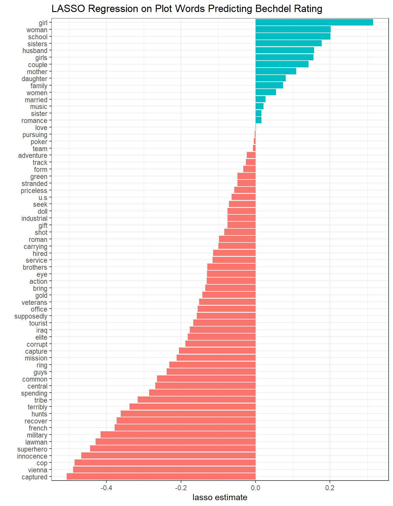
Now I can use the tidymoels meta-package to get the similar result. This part of analysis is inspired by Julia Silge’s blog post (link).
movie_wider <- movie_joined %>%
  mutate(row_id = row_number()) %>%
  unnest_tokens(word, plot) %>%
  anti_join(stop_words) %>%
  select(row_id, word, bechdel_rating) %>%
  filter(!is.na(word)) %>%
  mutate(value = 1) %>%
  distinct() %>%
  pivot_wider(names_from = "word",
              values_from = "value",
              values_fill = 0)

movie_wider
## # A tibble: 1,591 x 7,310
## row_id bechdel_rating antebellum united solomon northup free black upstate
## <int> <dbl> <dbl> <dbl> <dbl> <dbl> <dbl> <dbl> <dbl>
## 1 3 3 1 1 1 1 1 1 1
## 2 4 1 0 0 0 0 0 0 0
## 3 5 2 0 0 0 0 0 0 0
## 4 6 2 0 0 0 0 0 0 0
## 5 7 1 0 0 0 0 0 0 0
## 6 8 3 0 0 0 0 0 0 0
## 7 9 3 0 0 0 0 0 0 0
## 8 10 1 0 0 0 0 0 0 0
## 9 11 3 0 0 0 0 0 0 0
## 10 12 3 0 0 0 0 0 0 0
## # ... with 1,581 more rows, and 7,301 more variables: york <dbl>,
## # abducted <dbl>, sold <dbl>, slavery <dbl>, dea <dbl>, agent <dbl>,
## # naval <dbl>, intelligence <dbl>, officer <dbl>, run <dbl>, botched <dbl>,
## # attempt <dbl>, infiltrate <dbl>, drug <dbl>, cartel <dbl>, fleeing <dbl>,
## # learn <dbl>, secret <dbl>, shaky <dbl>, alliance <dbl>, undercover <dbl>,
## # life <dbl>, story <dbl>, jackie <dbl>, robinson <dbl>, history <dbl>,
## # signing <dbl>, brooklyn <dbl>, dodgers <dbl>, guidance <dbl>, ...movie_rec <- recipe(bechdel_rating ~ ., data = movie_wider) %>%
update_role(row_id, new_role = "ID")
movie_prep <- movie_rec %>%
prep(strings_as_factors = FALSE)set.seed(2022)
movie_boot <- bootstraps(movie_wider)
tune_spec <- linear_reg(penalty = tune(), mixture = 1) %>%
set_engine("glmnet")
lambda_grid <- grid_regular(penalty(), levels = 50)
doParallel::registerDoParallel(cores = 8)
set.seed(2022)
lasso_grid <- tune_grid(
workflow() %>%
add_recipe(movie_rec) %>% add_model(tune_spec),
resamples = movie_boot,
grid = lambda_grid
)
lowest_rmse <- lasso_grid %>%
select_best("rmse", maximize = FALSE)
finalize_workflow(
workflow() %>%
add_recipe(movie_rec) %>% add_model(tune_spec),
lowest_rmse
) %>%
fit(movie_wider) %>%
extract_fit_parsnip() %>%
vip::vi(lambda = lowest_rmse$penalty) %>%
mutate(Importance = if_else(Sign == "NEG", -Importance, Importance)) %>%
group_by(Sign) %>%
slice_max(abs(Importance), n = 10) %>%
ungroup() %>%
mutate(
Variable = fct_reorder(Variable, Importance)
) %>%
ggplot(aes(x = Importance, y = Variable, fill = Sign)) +
geom_col() +
scale_x_continuous(expand = c(0, 0)) +
labs(title = "Top 10 Most Important Variables") +
theme(legend.position = "none")
Words such as girl, woman, school etc. would contribute very positively to the bechdel score, but words like innocence, superhero etc. do the opposite effects.
Genres:
movie_joined %>%
  filter(!is.na(genre)) %>%
  separate_rows(genre, sep = ", ") %>%
  count(genre, binary, sort = T) %>%
  mutate(genre = fct_reorder(genre, n, sum)) %>%
  ggplot(aes(n, genre, fill = binary)) +
  geom_col() +
  labs(x = "# of movies",
       fill = "bechdel result",
       title = "Bechdel Result per Genre")