Vidoe Games Data Visualization
Sun, Mar 20, 2022
5-minute read
This blog post analyzes vidoe games time-series data from TidyTuesday. I personally never play video games and know nothing about them, but through data analysis in this post, I can use data to shed some light on what video games are popular over time and which games gained popularity during the COVID lockdown (March 2020).
Load the packages:
library(tidyverse)
library(lubridate)
library(scales)
library(tidytext)
theme_set(theme_bw())
Load and clean up the data:
games <- read_csv('https://raw.githubusercontent.com/rfordatascience/tidytuesday/master/data/2021/2021-03-16/games.csv') %>%
  rename(avg_player_num = avg,
         gain_from_pre_month = gain) %>%
  mutate(avg_peak_perc = as.numeric(str_remove(avg_peak_perc, "%"))) %>%
  left_join(tibble(month = month.name,
                   month_num = 1:12),
            by = "month") %>%
  select(-month) %>%
  rename(month = month_num,
         avg_peak_pct = avg_peak_perc,
         peak_num = peak) %>%
  relocate(month, .after = "year") %>%
  mutate(date = make_date(year, month),
         gain_from_pre_month = replace_na(gain_from_pre_month, 0),
         gamename = str_to_title(gamename))


games
## # A tibble: 83,631 x 8
## gamename year month avg_player_num gain_from_pre_m~ peak_num avg_peak_pct
## <chr> <dbl> <int> <dbl> <dbl> <dbl> <dbl>
## 1 Counter-St~ 2021 2 741013. -2196. 1123485 66.0
## 2 Dota 2 2021 2 404832. -27840. 651615 62.1
## 3 Playerunkn~ 2021 2 198958. -2290. 447390 44.5
## 4 Apex Legen~ 2021 2 120983. 49216. 196799 61.5
## 5 Rust 2021 2 117742. -24375. 224276 52.5
## 6 Team Fortr~ 2021 2 101231. 18083. 133620 75.8
## 7 Grand Thef~ 2021 2 90648. -10603. 146438 61.9
## 8 Tom Clancy~ 2021 2 72383. -5335. 113338 63.9
## 9 Rocket Lea~ 2021 2 53723. -5726. 103429 51.9
## 10 Path Of Ex~ 2021 2 46920. -766. 90539 51.8
## # ... with 83,621 more rows, and 1 more variable: date <date>Average # of players and peak # of players:
games %>%
  group_by(date) %>%
  summarize(across(c(avg_player_num, peak_num), mean),
            n = n()) %>%
  rename(`average player number` = avg_player_num,
         `peak player number` = peak_num) %>%
  pivot_longer(cols = 2:3) %>%
  ggplot(aes(date, value, color = name)) +
  geom_line() +
  geom_vline(xintercept = as.Date("2020-04-01"),
             lty = 2,
             color = "red") +
  geom_point(aes(size = n)) +
  scale_size_continuous(range = c(1,3)) +
  scale_x_date(date_breaks = "6 months",
               date_labels = "%y-%m") +
  labs(x = NULL,
       y = "# of players",
       color = NULL,
       size = "# of games",
       title = "Monthly # of Game Players",
subtitle = "The vertical line is the time when COVID lockdown taking place") 
Top 5 games with most players at the same time per year:
games %>%
  group_by(year, gamename) %>%
  slice_max(peak_num, n = 1) %>%
  ungroup() %>%
  group_by(year) %>%
  slice_max(peak_num, n = 5) %>%
  ungroup() %>%
  mutate(gamename = reorder_within(gamename, peak_num, year)) %>%
  ggplot(aes(peak_num, gamename, fill = factor(month))) +
  geom_col() +
  scale_y_reordered() +
  facet_wrap(~year, scales = "free_y") +
  theme(axis.text.x = element_text(angle = 90),
        strip.text = element_text(size = 15),
        plot.title = element_text(size = 18)) +
  labs(x = "peak player number",
       y = NULL,
       fill = "month",
       title = "Top 5 Games on Peak Numbers")
Games with most gains:
games %>%
  filter(gain_from_pre_month != 0) %>%
  group_by(date) %>%
  slice_max(abs(gain_from_pre_month), n = 1, with_ties = F) %>%
  ungroup() %>%
  mutate(group = if_else(gain_from_pre_month > 0, "pos", "neg")) %>%
  ggplot(aes(date, gain_from_pre_month, color = group)) +
  geom_line() +
  geom_point() +
  geom_text(aes(label = gamename), check_overlap = T,
            hjust = 1, vjust = 1) +
  theme(legend.position = "none") +
  labs(x = NULL,
       y = "gain from the previous month",
       title = "The Game with the Most Gains per Year and month",
       subtitle = "Both positive and negative are included")
Games with the largest average/peak:
games %>%
  group_by(date) %>%
  slice_max(avg_peak_pct, n = 1) %>%
  ungroup() %>%
  ggplot(aes(date, avg_peak_pct)) +
  geom_point(aes(size = peak_num)) +
  geom_line() +
  geom_text(aes(label = gamename),
            check_overlap = T,
            vjust = 1,
            hjust = 1,
            size = 3) +
  scale_y_continuous(labels = percent_format(scale = 1)) +
  labs(x = NULL,
       y = "avg / peak (%)",
       size = "peak number",
       title = "The Game with the Largest Average/Peak per Year per month") +
  expand_limits(x = as.Date("2010-01-01"))
Dota 2
games %>%
  filter(gamename == "Dota 2") %>%
  ggplot(aes(date, peak_num)) +
  geom_line() +
  scale_x_date(date_breaks = "1 year",
               date_labels = "%Y") +
  labs(x = NULL,
       y = "peak # of players",
       title = "Dota 2 Peak # of Players")
games %>%
  filter(fct_lump(gamename, n = 9, w = avg_player_num) != "Other") %>%
  mutate(gamename = fct_reorder(gamename, -avg_player_num, sum)) %>%
  ggplot(aes(date, avg_player_num, color = gamename)) +
  geom_line(show.legend = F, size = 1) +
  facet_wrap(~gamename, scales = "free_y") +
  scale_y_continuous(labels = comma) +
  labs(x = NULL,
       y = "average # of players",
       title = "Top 9 Games with the Largest Average # of Players")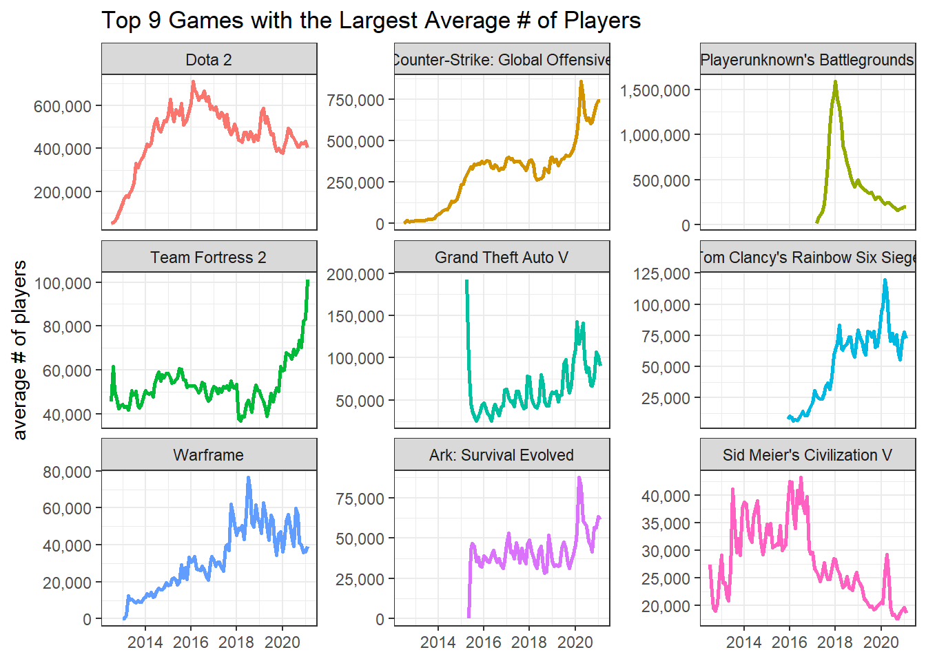
Which games got popular during the COVID lockdown?
games %>%
  filter(date >= "2018-01-01") %>%
  semi_join(
    games %>%
      filter(date == "2020-03-01") %>%
      slice_max(gain_from_pre_month, n = 9),
    by = "gamename"
) %>%
  mutate(gamename = fct_reorder(gamename, -avg_player_num, max)) %>%
  ggplot(aes(date, avg_player_num, color = gamename)) +
  geom_line(show.legend = F) +
  geom_vline(xintercept = as.Date("2020-03-01"),
             color = "red",
             lty = 2) +
  facet_wrap(~gamename, scales = "free_y")  +
  labs(x = NULL,
       y = "average # of players",
title = "Top 9 Most Gained Games during COVID Lockdown") 
games %>%
  group_by(date, gain_pos = gain_from_pre_month > 0) %>%
  summarize(n = n()) %>%
  ungroup() %>%
  add_count(date, wt = n, name = "total_game") %>%
  filter(gain_pos) %>%
  select(-gain_pos) %>%
  mutate(pct_gain = n/total_game) %>%
  ggplot(aes(date, pct_gain)) +
  geom_line() +
  scale_y_continuous(labels = percent) +
  scale_x_date(date_breaks = "1 year",
               date_labels = "%Y") +
  labs(x = "",
       y = "% of games gained users",
       title = "% of Games that Gained Users")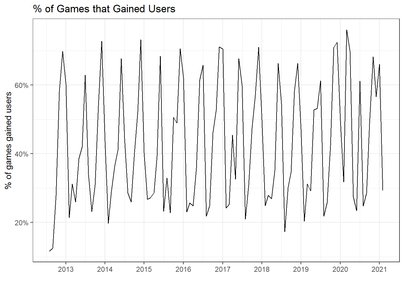
It seems like there is a seasonable pattern among the % of games that gained users.
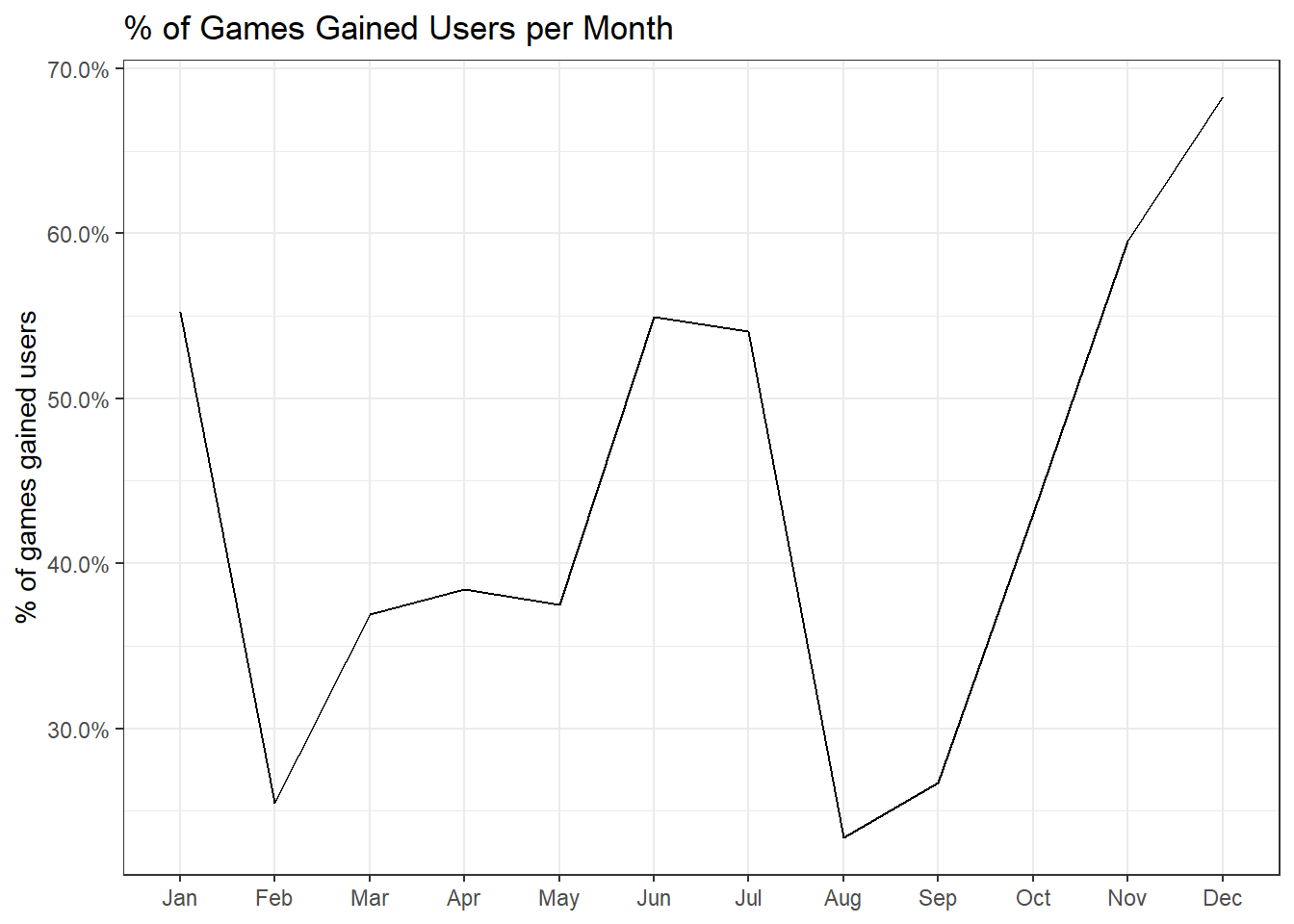
games %>%
  mutate(month = month(date, label = T),
         pos_gain = if_else(gain_from_pre_month > 0, TRUE, FALSE)) %>%
  group_by(month) %>%
  summarize(avg_pos_gain = mean(pos_gain)) %>%
  ggplot(aes(month, avg_pos_gain)) +
  geom_line(group = 1) +
  scale_y_continuous(labels = percent) +
  labs(x = NULL,
       y = "% of games gained users",
       title = "% of Games Gained Users per Month")