Deforestation Data Visualization
Deforestation is a contemporary topic nowadays, and in this blog post, I will analyze a few datasets from TidyTuesday to shed some light in this regard.
library(tidyverse)
library(scales)
library(worlddatajoin)
theme_set(theme_bw())
forest <- read_csv('https://raw.githubusercontent.com/rfordatascience/tidytuesday/master/data/2021/2021-04-06/forest.csv')
forest_area <- read_csv('https://raw.githubusercontent.com/rfordatascience/tidytuesday/master/data/2021/2021-04-06/forest_area.csv')
brazil_loss <- read_csv('https://raw.githubusercontent.com/rfordatascience/tidytuesday/master/data/2021/2021-04-06/brazil_loss.csv')
soybean_use <- read_csv('https://raw.githubusercontent.com/rfordatascience/tidytuesday/master/data/2021/2021-04-06/soybean_use.csv')
vegetable_oil <- read_csv('https://raw.githubusercontent.com/rfordatascience/tidytuesday/master/data/2021/2021-04-06/vegetable_oil.csv') %>%
mutate(crop_oil = str_remove_all(crop_oil, " \\(.+\\)$|,.+$"))brazil_loss %>%
pivot_longer(cols = 4:14,
names_to = "loss_reason",
values_to = "value") %>%
mutate(loss_reason = str_replace_all(loss_reason, "_", " "),
loss_reason = fct_reorder(loss_reason, -value, last)) %>%
ggplot(aes(year, value, color = loss_reason)) +
geom_line() +
geom_point() +
scale_x_continuous(breaks = seq(2000, 2013, 2)) +
scale_y_continuous(labels = comma) +
labs(x = NULL,
y = NULL,
color = "loss reason",
title = "Reasons Contributing to Brazilian Forest Loss per Year") 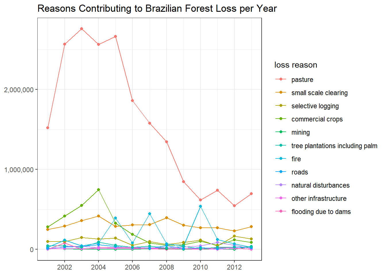
Over the years, the No.1 reason that contributed the forest loss in Brazil was the pasture loss, and it was way more than other factors.
soybean_long <- soybean_use %>%
  pivot_longer(cols = 4:6, names_to = "food_type") %>%
  mutate(food_type = str_replace(food_type, "_", " "))

soybean_long %>%
  filter(entity %in% c("Africa", "Asia", "Oceania", "Europe", "Americas")) %>%
  ggplot(aes(year, value, fill = food_type)) +
  geom_col(position = "dodge") +
  facet_wrap(~entity, ncol = 1) +
  scale_x_continuous(breaks = seq(1960, 2020, 10)) +
  labs(x = NULL,
       y = NULL,
       fill = "",
title = "How Soybean was Used Across 5 Continents?") 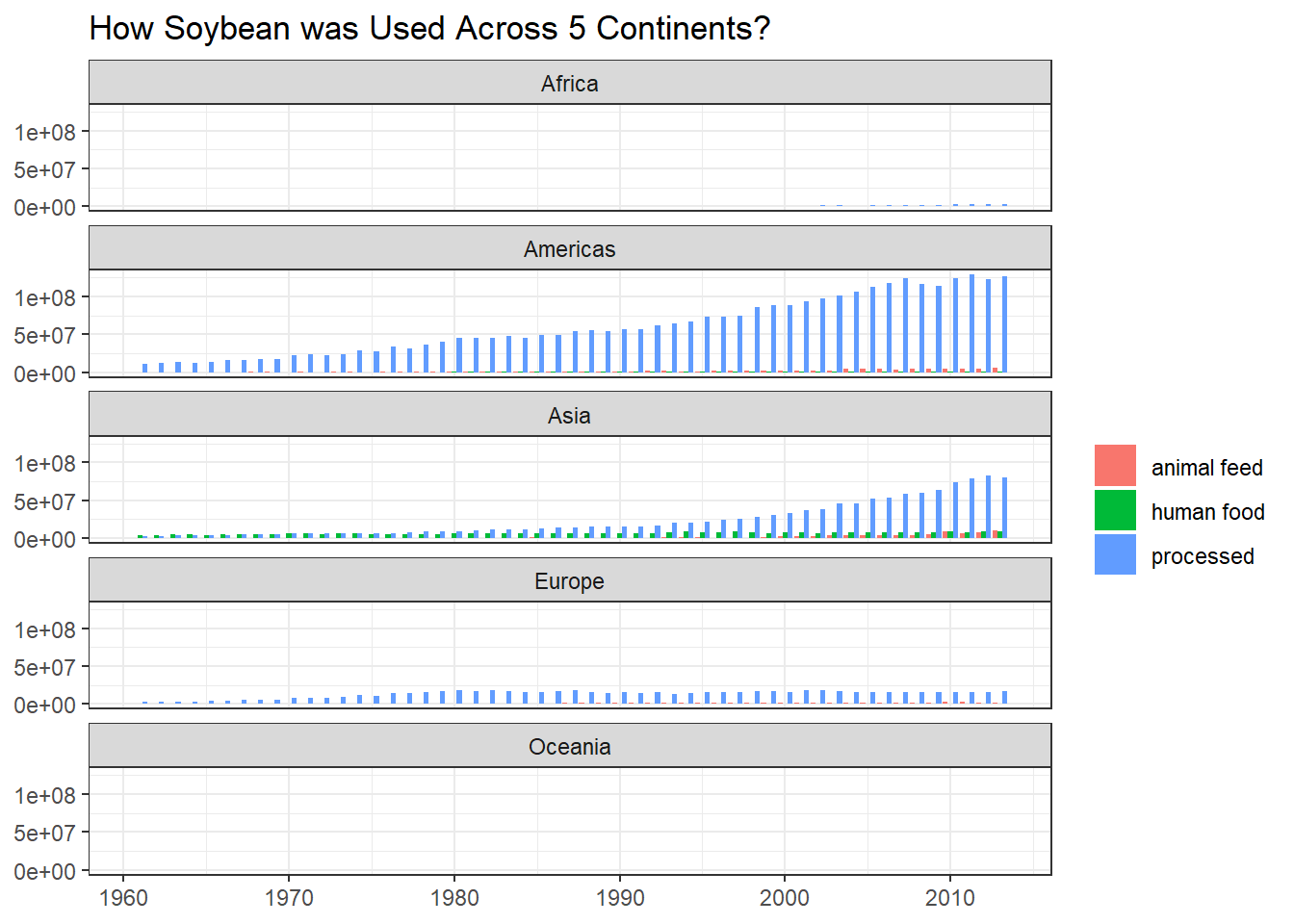
There was a growing trend on soybean being processed over the years in Americas and Asia, but in other three continents there was no such a clear trend when compared to the continents.
world_data_2013 <- world_data(2013)

soybean_map <- soybean_long %>%
  filter(year == 2013,
         !is.na(code)) %>%
  right_join(world_data_2013 %>%
              select(-year), by = c("code" = "iso3c"))

soybean_map %>%
  bind_rows(
    soybean_map %>%
      filter(is.na(food_type)) %>%
      mutate(food_type = replace_na(food_type, "animal feed")) %>%
      bind_rows(soybean_map %>%
                  filter(is.na(food_type)) %>%
                  mutate(food_type = replace_na(food_type, "human food"))) %>%
      bind_rows(soybean_map %>%
                  filter(is.na(food_type)) %>%
                  mutate(food_type = replace_na(food_type, "processed")))
  ) %>%
  filter(!is.na(food_type),
         region != "Antarctica") %>%
  ggplot(aes(long, lat, group = group, fill = value)) +
  geom_polygon() +
  theme_void() +
  facet_wrap(~food_type, ncol = 1) +
  coord_fixed() +
  scale_fill_gradient(low = "red",
                      high = "green") +
  theme(strip.text = element_text(size = 15),
        plot.title = element_text(size = 18)) +
  labs(x = "soybean produced in 2013",
       fill = NULL,
       title = "Soybean Production per Country and Its Usage")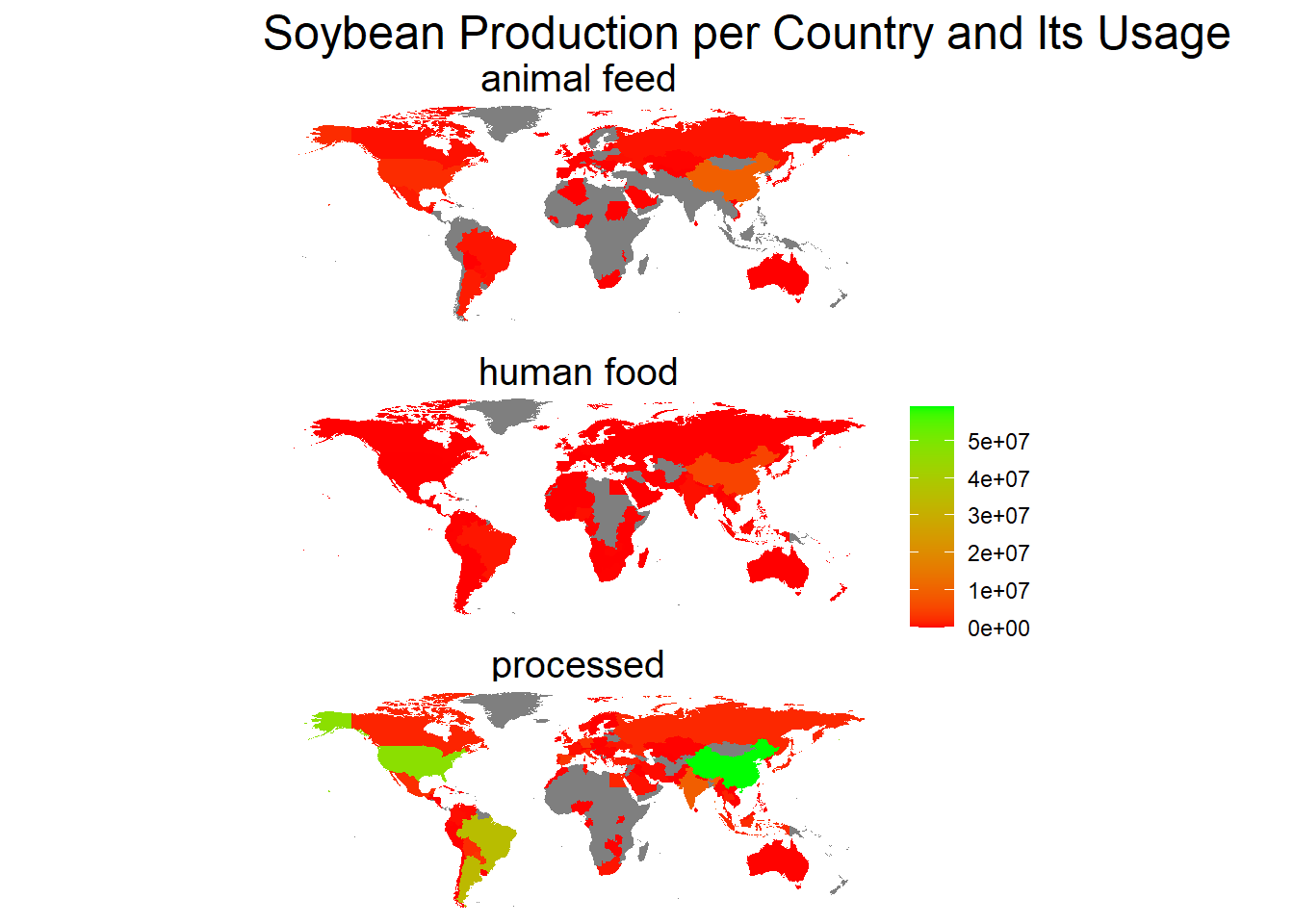
soybean_long %>%
  filter(entity == "World") %>%
  mutate(food_type = fct_reorder(food_type, -value, sum)) %>%
  ggplot(aes(year, value, color = food_type)) +
  geom_line() +
  geom_point() +
  scale_x_continuous(breaks = seq(1960, 2020, 10)) +
  labs(x = NULL,
       y = NULL,
       color = NULL,
       title = "World Soybean Usage per Year")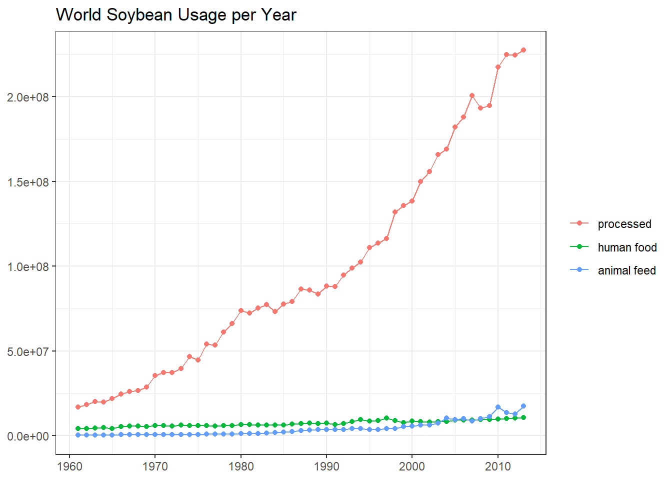
World vegatable oil:
vegetable_oil %>%
  filter(entity == "World") %>%
  mutate(crop_oil = fct_lump(crop_oil, n = 5, w = production)) %>%
  group_by(year, crop_oil) %>%
  summarize(production = sum(production)) %>%
  ungroup() %>%
  mutate(crop_oil = fct_reorder(crop_oil, -production, last)) %>%
  ggplot(aes(year, production, color = crop_oil)) +
  geom_point() +
  geom_line() +
  scale_x_continuous(breaks = seq(1960, 2020, 10)) +
  labs(x = NULL,
       y = "production (tonnes)",
       color = "crop",
title = "Crop Oil Production") 
The countries with most production of vegetable oil:
vegetable_oil %>%
  filter(!is.na(production),
         entity != "World",
         !is.na(code)) %>%
  filter(fct_lump(crop_oil, n = 3, w = production) != "Other") %>%
  group_by(year, crop_oil) %>%
  slice_max(production, n = 1) %>%
  ungroup() %>%
  mutate(crop_oil = fct_reorder(crop_oil, -production, last)) %>%
  ggplot(aes(year, production, color = crop_oil)) +
  geom_line() +
  geom_point() +
  geom_text(aes(label = code), hjust = 1, vjust = 1, check_overlap = T, size = 3) +
  scale_x_continuous(breaks = seq(1960, 2020, 10)) +
  labs(x = NULL,
       y = "production (tonnes)",
       color = NULL,
       title = "The Countries with the Most Vegetable Oil Production per Year")
Forest net conversion:
forest %>%
  left_join(
    world_data_2013 %>%
      distinct(country, iso3c, continent),
    by = c("code" = "iso3c")
  ) %>%
  filter(!is.na(continent)) %>%
  ggplot(aes(net_forest_conversion, continent, fill = factor(year), color = factor(year))) +
  geom_boxplot(alpha = 0.6) +
  geom_text(aes(label = country),
            hjust = 1,
            vjust = 1,
            check_overlap = T) +
  labs(x = "net forest conversion (in hectares)",
       y = NULL,
       fill = NULL,
       title = "Net Forest Conversion per Year per Continent") +
  scale_color_discrete(guide = "none")
China made significant effort to recover forest in 1990 and 2000.
forest_area_continent <- forest_area %>%
  left_join(
    world_data_2013 %>%
      distinct(country, iso3c, continent),
    by = c("code" = "iso3c")
  ) %>%
  select(-country) %>%
  filter(!is.na(continent))

forest_area_continent %>%
  group_by(year, continent) %>%
  summarize(forest_area = sum(forest_area)) %>%
  ungroup() %>%
  ggplot(aes(year, forest_area, fill = continent)) +
  geom_col() +
  scale_y_continuous(labels = percent_format(scale = 1)) +
  labs(x = NULL,
       y = "% of forest area",
       fill = NULL,
       title = "% of Forest Area per Continent")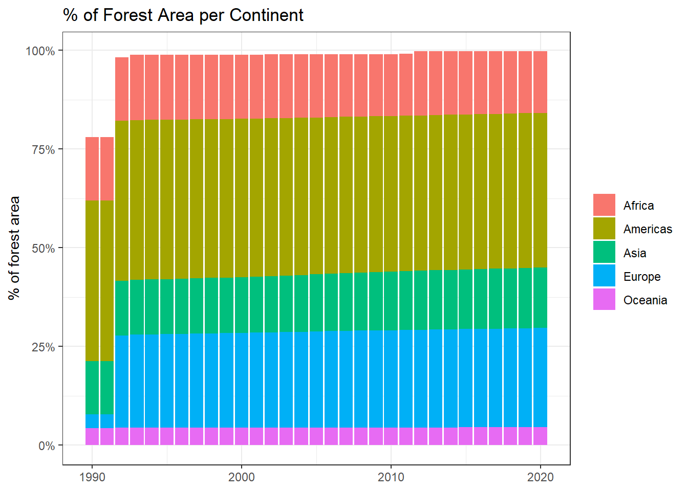
There is some data issue in the first two years, as they are not added up to 100%. Other than that, there was no significant change on forest area, although it is worth noting that Asia had experienced an increase in the statstic over the years.